How is wealth distributed across British households? Reassessing the valuation of pensions

Executive summary

Reliable statistics on the distribution of wealth – and how this has changed over time – are essential for informing a range of policy debates. Unfortunately, current official statistics from the Office for National Statistics (ONS) do not provide a coherent or consistent guide to how wealth is distributed. They are based on the Wealth and Assets Survey (WAS) – the only dataset aiming to comprehensively measure the distribution of wealth in Great Britain – yet they contain important inconsistencies over time. These inconsistencies arise due to the recent methodological changes to the valuation of households’ private pension wealth, introduced in Round 8 of the data (covering 2020–22), but not applied to previous versions of data (covering 2006 to 2020).

In addition, both before and after the methodological changes, the ONS values much of private pension wealth in a way that is fundamentally incompatible with how other assets are valued in the survey (as first pointed out in Adam et al. (2025)). This results in inconsistent comparisons for groups who hold more and less of their wealth in these types of pensions, distorting the measured distribution of wealth.

In this report, we propose an improved measure of private pension wealth (the single largest component of household wealth in Great Britain) that can be calculated coherently and consistently over time in WAS. We apply this measure to all editions of the data to uncover new insights about how wealth is distributed across Great Britain, and how this has changed over time.

1. Introduction

How wealthy is the average British household? How is wealth distributed across the population? And have households become wealthier over time? The answers to such questions are important to understanding both our economy and our society, as well as for considering the merits of a range of policies. But data that might help us to answer them are scarce. Only one official survey, the Wealth and Assets Survey (WAS), aims to directly and comprehensively measure household wealth in Great Britain. That stands in stark contrast to income, information on which is not only collected in a wide range of government surveys but also leaves its imprint in the administrative records of the tax and benefit system.

To add to this difficulty, WAS has undergone a number of major methodological changes since its inception in 2006. The most substantial of these relate to the valuation of private pension wealth, which in most years is the single largest component of households’ measured total wealth (closely followed by housing). The magnitude of these methodological changes has in some cases been very large. The most recent revision – affecting data from April 2020 onwards – subtracted a staggering £2.3 trillion from measured household private pension wealth and was applied without constructing a consistent back-series, introducing serious difficulties in comparing data over time. Worse, a number of the revisions have been ill judged, leading to serious flaws in how pension assets are valued (Adam et al., 2025). The result is that little can now be said with confidence about how wealth is distributed in Great Britain and how this has changed over time.

In this report, we seek to ameliorate this situation. We use an improved approach to valuing private pension wealth to produce new estimates of the distribution of wealth in Great Britain and how it has evolved over time. Section 2 outlines the main shortcomings of the current WAS methodology and the adjustments we propose to mitigate them. Section 3 presents our new estimates of how wealth is distributed across several dimensions. Section 4 offers a brief conclusion. The code to implement our improved valuation approach is available online here: https://github.com/laurenceob/was-pension-wealth.

2. How should pension wealth be valued?

We begin this section by setting out the principles of estimating the market value of different types of pensions. We then discuss how the Wealth and Assets Survey (WAS) currently implements these valuations, and how this has changed over time. Finally, we discuss the problematic aspects of the valuation methodology currently used by the Office for National Statistics (ONS) in WAS, before setting out our methodology and the advantages of this approach.

Principles of pension valuation

The Wealth and Assets Survey measures household wealth in Great Britain by asking survey respondents about the value of wealth held in various forms.1 For the most part, this involves eliciting the price that assets would be expected to sell for on the open market at the time of the survey interview. For many assets, this is conceptually straightforward: for example, to value housing assets, people are asked: ‘About how much would you expect to get for your current home if you sold it today …?’ (UK Data Service, undated).

Valuation of some assets, however, is not so simple. Private pensions2 pose a particular problem because – unlike houses, cars, listed equities, corporate or government bonds, or fine art – they cannot be bought and sold. With no market price available, their value must instead be estimated. It should be noted from the outset that, in order to produce a valuation that is consistent with other assets in WAS (and which can therefore be added to these values to produce an estimate of total wealth), it is the market value of pensions that must be estimated. In other words, the valuer must seek to answer the following question: ‘How much could a pension be sold for if sale were permitted?’.

Exactly how valuation is to be undertaken depends on the characteristics of the pension being valued. Broadly speaking, private pensions in the UK can be broken down into two categories: defined contribution (DC) and defined benefit (DB). DC pensions involve making contributions into a pot which is then invested in a range of assets, and whose value depends on the amounts contributed and the investment returns achieved. DB pensions, on the other hand, typically involve an employer promising to pay an employee a percentage of their final or career-average salary every year from a set retirement age until death, with that percentage rising in line with the number of years that the employee remains in the scheme. DB pensions are particularly common for people currently working in the public sector, but historically many private sector workers also built up entitlement to a DB pension. In addition, the valuation process differs depending on whether the individual has started to draw income from the pension or not.

For DC pension pots that have not been accessed, a relatively straightforward approach to estimating market value is available: simply taking the current market value of the assets held in the pension fund.3

Valuing DB pensions is more complicated as they are not a stock of assets, but rather a promise of future income. Broadly speaking, for DB pensions not in payment, this valuation can be thought of in three steps, the second and third of which both involve ‘discounting’ – that is, converting future sums of money into today’s terms. The idea behind discounting is that receiving £1,000 today is not of equal value to receiving £1,000 in 10 years’ time. One way to think of this is that £1,000 today could be saved in an asset with little to no risk (e.g. through the purchase of government bonds) and grow by virtue of the interest payments received. For example, an investment of £1,000 earning a 2% annual return would grow to be worth a little over £1,200 in 10 years’ time. In this example, a claim to £1,200 in 10 years’ time would therefore have a market value of £1,000 today. Future sums must therefore be ‘discounted’ (i.e. scaled down) by some market interest rate to determine their value in today’s terms.

The three steps into which the valuation of DB pensions can be broken down are:

1. Calculate the annual retirement income that has been promised. Given enough information about the scheme in question (and the salary of the recipient), this is mostly a matter of arithmetic,4 though in practice the difficulty of eliciting all the necessary information in a survey means that some simplifying assumptions are generally required.5
2. Convert that promised income into a lump-sum equivalent received at retirement.6 This is typically done through an ‘annuitisation’ procedure: calculating the price of an annuity (a financial instrument that provides a regular income, guaranteed until death) that would pay out the same income as the pension from the normal retirement age (the age at which the pension can begin to be drawn in full) onwards. This lump-sum conversion embeds two key inputs: the life expectancy of the scheme member7 and a discount rate for the post-retirement period. The result is an estimate of the cash amount that, if received at retirement, would be of equivalent value to the promised stream of pension income.
3. Convert that future income into today’s terms. The lump-sum equivalent calculated in step 2 represents a value at the point of retirement, which may be many years away. It must therefore be discounted over the period between the individual’s current age and their normal retirement age to arrive at its market value today.

If undertaken correctly,the process above will provide a coherent estimate (subject to the caveats outlined in Appendix A) of the market price a DB pension would be expected to command were it tradable.

One final form of pension wealth that must be considered is pensions in payment (whether DB or DC). In these cases, the promised income is already known and is already being received and so steps 1 and 3 are superfluous. Valuation therefore requires following only step 2 of the above approach.

How are pensions valued in the Wealth and Assets Survey?

Two major changes in methodology have occurred in how WAS undertakes these steps to value pension assets. The first major change occurred in the third wave of the survey (covering July 2010 to June 2012), following which the ONS retrospectively modified the calculation of pension wealth in Waves 1 and 2 to ensure that the series remained consistent over time.8 The second major change occurred in Round 8 (the most recent vintage of the data at the time of writing, covering April 2020 to March 2022). The ONS has not, at the time of writing, applied this methodology to previous editions of WAS, leading to a structural break in the time series. In this subsection, we outline how pensions are valued in WAS and how the valuation method has changed over time.

Throughout, different valuation methods are used depending on whether the scheme is DB or DC and whether the scheme member is in receipt of a regular income from their pension. For DC pensions where the member had not yet begun receiving a regular income (e.g. because they had not yet reached retirement age), the valuation methodology has not changed over time: the pension’s value is simply set equal to the amount held in the pension pot. For DB pensions not yet in payment, the ONS implements the three-step procedure described in the previous subsection: calculating the promised retirement income (step 1), converting it into a lump-sum equivalent at retirement (step 2) and discounting that lump sum back to today (step 3). For pensions already in payment (whether DB or DC), only step 2 is required, applied at the respondent’s current age.

There are three key aspects of this method that have changed over time: the estimate of the respondent’s normal retirement age (an input into steps 2 and 3), the method of lump-sum conversion (step 2) and the discount rate applied to the pre-retirement period (step 3). The remainder of this subsection describes the changes to each of these aspects in turn.

Normal retirement age

In order to elicit normal retirement ages (the age at which a DB pension income can begin to be drawn in full), WAS respondents are asked: ‘What is the earliest age you can draw a pension from this scheme?’.9 This wording is potentially problematic because DB pensions typically allow scheme members to begin drawing from their pension before the normal retirement age in return for accepting a reduced pension income. If this earlier age is confused for the normal retirement age, it will tend to make DB pensions look like they provide a full income for longer, leading their value to be overstated. As discussed in Adam et al. (2025), this ambiguity led the ONS to amend its approach by imposing the blanket assumption that the holders of DB pensions are able to begin drawing their full pension no earlier than age 60 from Round 8 of WAS onwards. This change was not applied retrospectively and so contributes to the structural break in the WAS data from Round 8 onwards. To give a sense of scale, the ONS estimated that this change reduced the total measured value of pension wealth in Round 7 of WAS by roughly £300 billion, or around 5% (Office for National Statistics, 2024b).

Lump-sum conversion

Prior to Round 8, the annuity prices used in step 2 by the ONS were taken from the annuity market at the time of the survey. Specifically, it used the market price of an annuity offering the same stream of income as the pension being valued. From Round 8 of WAS onwards, the ONS ceased using market annuity prices, electing instead to use annuity rates calculated directly by the Government Actuarial Department (GAD). These annuity rates are in spirit similar to the prices used in previous waves but require GAD to make explicit choices as to the discount rate and longevity estimates that are used. The discount rate chosen by GAD was the Superannuation Contributions Adjusted for Past Experience (SCAPE) rate – an estimate of UK GDP growth in the medium term. While there are advantages to using directly calculated annuity prices rather than current market annuity prices, the choice of the SCAPE rate was not a welcome one, as we discuss in the next subsection. The scale of this change was very substantial, reducing the measured value of pension wealth in Round 7 of WAS (covering the period April 2018 to March 2020) by £2.3 trillion or 36%.

Pre-retirement discounting

In the initial methodology, used in the first two waves of the survey, discounting of the pre-retirement period for DB pensions not yet in payment was undertaken using a real interest rate based on AA corporate bond rates. The methodology introduced in the third wave of WAS (but then retroactively applied to the first two waves) instead used the (nominal) SCAPE rate. Because the discount rate was nominal (i.e. included inflation), it effectively ignored the fact that DB pensions are typically inflation-protected (see Adam et al. (2025) for further discussion of this point). In Round 8, the ONS therefore changed its approach once more, stripping out inflation and applying the real SCAPE rate to the pre-retirement period. This change increased the total measured value of pension wealth in Round 7 of WAS by £500 billion, i.e. around 8%.

Problems with the current ONS approach

The methodological changes introduced in Round 8 of WAS contained a number of welcome improvements. The change to the estimation of normal retirement ages is a clear improvement: before this change, a large number of respondents were treated as being able to begin drawing their full pension implausibly early, leading to an overestimation of their pension wealth. Similarly, the move from a nominal to a real discount rate was welcome, as using a nominal rate effectively ignored the inflation protection that DB pensions typically provide, missing a substantial part of their value (particularly where the individual is still a long way from retirement).

However, two serious problems remain. First, the improvements made in Round 8 have not been applied to previous editions of WAS, introducing a structural break into the time series. This makes it impossible to draw reliable comparisons of wealth over time using official statistics.

Second, and most fundamentally, the continued use of the SCAPE rate for discounting is deeply flawed, both as the pre-retirement discount rate and as the basis for the directly calculated annuity prices introduced in Round 8. This is because the SCAPE rate is not in any meaningful sense a rate of interest. Rather, it is a government-published rate principally used to determine the level of contributions that public sector employers must make to the Treasury in respect of their DB pensions promises to their employees. Crucially, it is based not on the prevailing rate of interest in the market but on medium-term forecasts of the rate of UK GDP growth.10 That makes it a fundamentally inappropriate tool for converting the value of a future income into today’s terms. What would be the market price today of the promised future pension benefit? To answer that, what matters is the market interest rate, not the rate of GDP growth in the medium term.

This matters in practice because market interest rates affect the market prices, and therefore the measured value, of other assets in WAS (such as housing and financial assets). Changes in market interest rates will thus shift the values of other assets but not, under SCAPE-based discounting, the values of future pension benefits. This is despite the fact that the fundamental principles of asset pricing suggest that the market value of future pension benefits would respond to market interest rates (Cochrane, 2005). SCAPE-based discounting therefore introduces an inconsistency in the treatment of different types of wealth, distorting comparisons of households whose portfolios differ in the share held in private pensions. If market interest rates do not enter into the estimated value of pensions then when market interest rates change the market value of all other assets in WAS (from housing to shares to government bonds) will change, while that of pensions will not. That will lead to an inaccurate picture of the relative wealth of individuals, making those whose wealth is more concentrated in pensions seem more or less wealthy than those whose wealth is more concentrated in, say, housing.

The result is that statistics currently derived from WAS cannot be considered a reliable guide to the distribution of household wealth or to how this has changed over time.

Our proposed methodology

We therefore propose a new approach to the valuation of pension assets. Our approach sets out both to make what we believe to be a more coherent set of methodological choices, and to apply those choices consistently over time. In this subsection, we describe the most significant way in which our approach differs from that taken in previous editions of WAS. A more comprehensive account of our methodology is provided in Appendix A, while code allowing researchers to implement our methodology can be downloaded here: https://github.com/laurenceob/was-pension-wealth.

Normal retirement age

Our methodology applies the improvement made by ONS in Round 8 – imposing a minimum normal retirement age of 60 – to all previous vintages of the survey, removing one source of the structural break in the time series.

Lump-sum conversion

A central choice to make is whether lump-sum conversion should be undertaken using market annuity prices (as used in WAS prior to Round 8) or ‘directly calculated’ annuity rates (as used in Round 8 of WAS). While both approaches have merits, we elect to use directly calculated annuity rates for two main reasons.

First, for valuing DB pensions that are not yet in payment, contemporaneous market annuity prices may not be a good representation of the annuity price an individual might expect to receive when they decide to draw on their pension wealth in the future. This is due to both differences in life expectancy between cohorts retiring now and in the future, and differences in the expected path of future market interest rates (which are embedded in annuity prices) now and in the future.

Second, there are concerns that UK annuity markets suffer from adverse selection – that is, annuities are disproportionately purchased by individuals who expect to live longer than average. There is empirical evidence for this even prior to the introduction of pension freedoms in 2015 (which ended the near-mandatory purchase of annuities for DC pension holders) (Finkelstein and Poterba, 2004), and the problem is likely to have been exacerbated since. This means that market annuity prices will reflect the characteristics (e.g. expected longevity) of those who choose to buy annuities rather than of the general population.

Directly calculated annuity rates allow us to sidestep these issues with observed market annuity prices. For any given respondent, born in a given year and with a given normal retirement age, we calculate annuity prices based on the typical life expectancy of someone born in that year and based on the expected path of future market interest rates starting from their normal retirement age (our choice of interest rate is described in detail below).

Choice of discount rate

Where our method departs most significantly from that used in the most recent edition of WAS is in the choice of discount rate, used in converting future income into today’s terms, and underlying our calculation of annuity prices. As set out in the previous subsection, the SCAPE rate is not an appropriate rate for such a conversion; indeed, it is not an interest rate at all. In place of SCAPE, our methodology instead makes use of the market interest rate for government debt (the ‘gilt’ rate).11 As discussed in Box 1 at the end of this section, using this rate leads to a much more coherent estimate of the market value of DB pension assets if they were tradable.

Using the real interest rate on government debt to discount future pension incomes is not a novel approach. Recent estimates of the distribution of wealth in the United States published by the Congressional Budget Office (Karamcheva and Perez-Zetune, 2023) make use of a similar method (although, naturally, the yield chosen is that on US Treasury bonds, not UK gilts).12 Novy-Marx and Rauh (2011) also take market interest rates on US government debt (both local and federal) as the basis for discounting future DB pension liabilities.

A corollary of our choice to use gilt-based discounting is that the estimated value of pension wealth will rise and fall in response to changing interest rates. This is not the case for the most recent iteration of the ONS methodology (where SCAPE-based discounting is used with the explicit aim of ensuring pension wealth is insensitive to changes in market interest rates) and is only partially true in earlier editions of WAS (where market annuity prices used to value pension income after retirement implicitly embed market interest rates). As discussed in the previous subsection, we consider this responsiveness to be one of the key advantages of our approach, as it makes the valuation of pension wealth consistent with how other types of assets are valued in WAS.

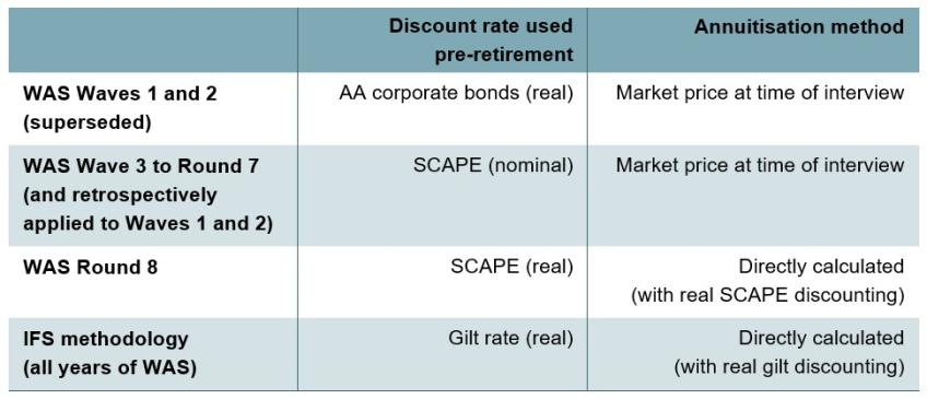
Table 1 shows how the discount rates and annuitisation methods differ between our methodology and different versions of the WAS methodology.

Table 1. Summary of approaches to pension valuation

Outstanding issues

While we consider the methodology developed for this report to be the most coherent approach currently available for valuing pension wealth in WAS, it should by no means be seen as the last word on the subject. Appendix A sets out a number of outstanding issues regarding the way in which pension wealth is valued in WAS and there remains considerable scope for future research to make further improvements to measurement.

Nor are potential improvements to methodology limited to the measurement of pension wealth. Recent evaluations suggest, for example, that respondents appear to systematically overestimate the value of housing in WAS (Office for National Statistics, 2024a), while sections of the WAS questionnaire relating to business assets have changed materially over time, making consistent measurement difficult. Meanwhile, Advani, Bangham and Leslie (2021) have shown that WAS struggles to comprehensively capture the very top of the wealth distribution.

3. New estimates of household wealth in Great Britain

In this section, we set out how the methodology proposed in the previous section alters the measured level, trend and distribution of household wealth over time when compared with the ONS methodology that currently underpins pension values in the Wealth and Assets Survey.

One major difference between the estimates produced by our proposed methodology and that of the Office for National Statistics is in the average level of measured household pension wealth. When applied to the most recent round of WAS data (2020–22), our methodology approximately doubles mean measured household pension wealth, from £230,000 to £450,000.19 Adding in other components of wealth – that is, housing, financial and physical wealth20 – we find that mean measured total household wealth was 37% higher under our methodology: £830,000, compared with £600,000 under the ONS methodology. In aggregate, this implies an increase in total measured household wealth from £16.3 trillion to £22.3 trillion. Note that we exclude business wealth in both measures due to inconsistencies in how it is recorded over time. We also make no adjustment for the fact that WAS likely underestimates household wealth at the very top of the distribution, as shown by Advani, Bangham and Leslie (2021).

The gulf between average measured pension wealth under the two methodologies occurs as a result of the different discount rates used to value future pension incomes. Market interest rates (and specifically market interest rates on UK government debt, which underpin our methodology) were extremely low between April 2020 and March 2022. On average, a 15-year inflation-linked government bond purchased in this period yielded a real-terms interest rate of
–1.9% a year to the purchaser.21 That is, interest rates were so low that investors were prepared to settle for a return that did not even keep up with inflation. On the other hand, the SCAPE rate underpinning the ONS methodology was set at a fixed real rate of 2.4% throughout the period.22 This highlights the fundamental difference between the two approaches. Our methodology responds to low interest rates by increasing the estimated value of defined benefit pension promises (because a larger amount would need to be invested in order to yield the promised amount in the future) while the ONS approach does not.

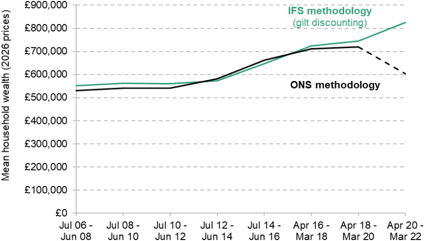
Figure 1 shows the mean level of total household wealth (in 2026 prices) over time, as estimated by the ONS and our methodologies. We indicate the series break in the ONS methodology for calculating pension wealth between 2018–20 and 2020–22 with a dotted line.

Figure 1. Mean household wealth over time by methodology

_{Note: Dashed line shows series break in ONS methodology.}

_{Source: Authors’ calculations using Wealth and Assets Survey, Waves/Rounds 1–8.}

As Figure 1 shows, both measures of mean total household wealth are remarkably similar prior to the recent change to the ONS methodology. Mean total household wealth increased under both measures by around 35% between 2006–08 and in 2018–20: from £530,000 to £720,000 under the ONS approach compared with an increase from £550,000 to £750,000 under our approach. This may initially seem surprising given that for 2020–22 there is only one substantive difference between the two methodologies (namely, the choice of discount rate), while in earlier years the two approaches are in some ways less similar. Prior to 2020–22, however, the methodological differences between the ONS approach and our approach push in different directions. On the one hand, the ONS measure applies a higher discount rate (the nominal SCAPE rate) to the period prior to retirement – reducing pension values relative to our methodology. On the other, the market annuity prices used in the previous ONS methodology implicitly apply a lower discount rate to the period following retirement – increasing pension values relative to our methodology.23 The net result is that, while the previous ONS methodology was undoubtedly flawed, the differences relative to our methodology had largely offsetting effects at the aggregate level.24

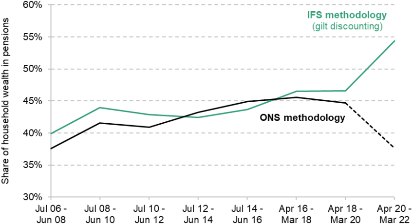
The share of household wealth held in pensions over time, shown in Figure 2, is consistent with the trends in mean wealth. The figure shows that the share of wealth in pensions was relatively similar under the two methodologies prior to the latest round of data, rising from around 40% in 2006–08 to around 45% in 2018–20. However, a large gap opened up in 2020–22, with the share of wealth in pensions rising to 54% under our methodology, but falling to 38% under the ONS methodology.

Figure 2. Share of household wealth in pensions over time by methodology

_{Note: Dashed line shows series break in ONS methodology.}

_{Source: Authors’ calculations using Wealth and Assets Survey, Waves/Rounds 1–8.}

Looking forwards, an important point to note is that market interest rates increased sharply over the course of 2022 and have (at the time of writing) remained elevated ever since. This is shown explicitly in Figure 3. The SCAPE rate, meanwhile, saw its most substantial reduction to date in 2023, from CPI+2.4% to CPI+1.7%. All else equal, this implies that our methodology would be expected to show a substantial decline in measured pension wealth in the 2022–24 edition of WAS (because rising real interest rates on gilts mean that promises of future pension incomes are less valuable), while the ONS methodology would be expected to record an increase in measured pension wealth (because of the reduction in the real SCAPE rate). The discrepancy between the two measures will therefore be considerably smaller in 2022–24 than in 2020–22.

Figure 3. Discount rates over time

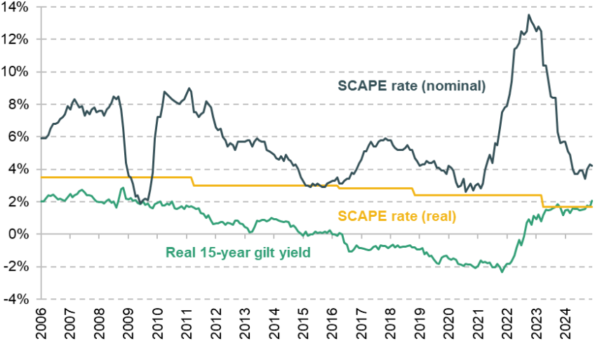
_{Note: Changes to the real SCAPE rate are shown at the time they were announced by the government, rather than when they came into effect for the purpose of valuing employer contributions to public service pensions. Real SCAPE rate is equal to (nominal) SCAPE rate minus RPI inflation rate before April 2011 and SCAPE rate minus CPI inflation rate from April 2011. Note that in the IFS methodology, discounting uses real gilt yields at different maturities depending on the horizon. We plot real yields on 15-year gilts to provide an approximate indication of the discount rates used.}

_{Source: Bank of England monthly government liability curve (real): archive data, available at https://www.bankofengland.co.uk/statistics/yield-curves. RPI and CPI rates from https://www.ons.gov.uk/economy/inflationandpriceindices.}

At a more fundamental level, it is worth pausing to consider what it means for average household wealth to change over time. On the face of it, the question may seem obtuse, but the role of interest rates in shaping asset values provokes difficult questions. This is not just an issue for defined benefit pensions: interest rates are a key driver of asset prices across essentially all forms of wealth. Is an increase in average wealth precipitated purely by a fall in interest rates properly interpreted as households becoming better off, on average, over time? After all, in a nation where all residents own houses and nothing else, a fall in interest rates that increases house prices will register as an increase in wealth, and yet the real resources at the country’s disposal will not have changed. Given the large changes in market interest rates since 2006, caution is required in the interpretation of statistics such as those shown in Figure 1.25

Where interest-rate-induced wealth changes do have an unambiguous impact is on the relative distribution of wealth. For example, an individual who owns a house that increases in value thanks to a fall in interest rates will become relatively more wealthy in a meaningful sense than someone whose wealth is held entirely in cash. This is because the person with a more valuable house can now sell their house for more cash, allowing higher consumption today, while cash-holders see no comparable gain. Given this, and the fact that a key advantage of the WAS data (relative to other available figures) is to provide insights into how wealth is distributed across individuals and households, the remainder of this section focuses on how methodological choices impact the relative wealth of different groups of households and individuals.

How is household wealth distributed?

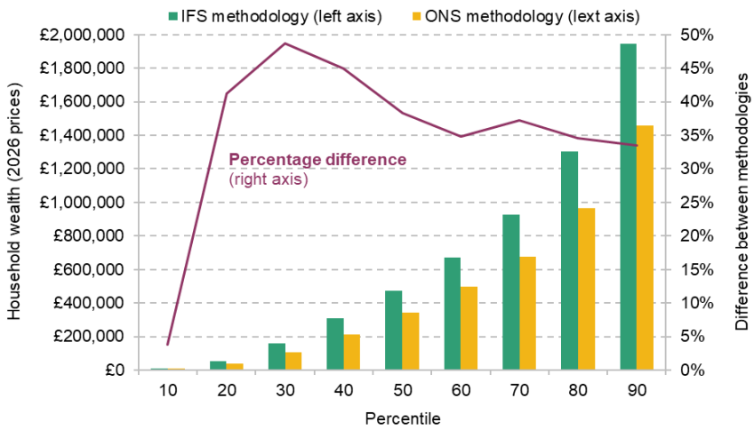
Figure 4 begins to shed light on this question by comparing the level of wealth at different points of the household wealth distribution in the latest edition of WAS using the ONS and our valuation methods. As would be expected (given the higher level of measured aggregate private pension wealth in this year), wealth is substantially higher across the distribution when the IFS methodology is used, with the largest increases in cash terms at the top of the distribution. At the 90th percentile, for instance, we value total household wealth in 2020–22 at £490,000 higher than official statistics.26 At the 50th percentile (i.e. the median), meanwhile, the increase in measured household wealth as a result of our method is only around £130,000. However, the percentage increase in measured household wealth is slightly higher towards the bottom of the distribution (except for the bottom 10%, who hold very little wealth under either measure). Households at the 30th percentile see a 49% increase in measured wealth under the IFS measure, compared with just a 34% increase for households at the 90th percentile.

Figure 4. Distribution of household wealth in the Wealth and Assets Survey Round 8 (April 2020 to March 2022), by methodology

_{Source: Authors’ calculations using Wealth and Assets Survey, Waves/Rounds 1–8.}

Despite this, the share of wealth held by the wealthiest 10% of households in 2020–22 is virtually identical under the two methodologies, at 42%. Ultimately, even though the IFS measure leads to a slightly larger proportional increase in wealth in the bottom half of the distribution than at the top, the bottom half holds so much less wealth than the top 10% to start with that the change in methodology has a very small impact on the top 10% share. The main effect of the IFS approach is therefore to widen absolute gaps in wealth between the top 10% and the rest of the distribution.

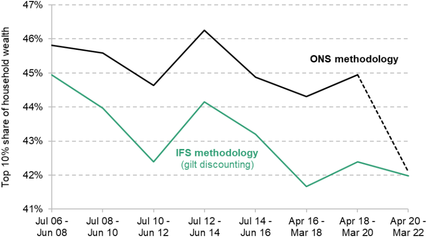
Figure 5 shows how the top 10% wealth share has evolved over time under both methodologies. Note that we continue to define total wealth as the sum of financial, housing, physical and pension wealth – that is, we exclude business wealth, which is particularly concentrated at the top of the distribution – and we also make no adjustment for potential under-reporting of wealth towards the top of the distribution (Advani, Bangham and Leslie, 2021).

Figure 5. Top 10% share of household wealth over time by methodology

_{Note: Dashed line shows series break in ONS methodology.}

_{Source: Authors’ calculations using Wealth and Assets Survey, Waves/Rounds 1–8.}

As Figure 5 makes clear, the ONS methodology registers slightly higher levels of wealth inequality than our measure in the period prior to 2020–22 (where the two measures produce similar estimates of aggregate wealth). The top 10% wealth share also shows a stronger downward trend under our methodology, falling from 45% in 2006–08 to 42% in 2018–20, compared with a fall from 46% to 45% under the ONS methodology. These results somewhat alter the broad narrative of how household wealth inequality has evolved in Great Britain over recent decades. Instead of a fairly stable share of wealth being held by the top 10% (as found by Advani, Bangham and Leslie (2021)), our measure of pension wealth points to this measure of household wealth inequality having declined moderately across the period for which WAS data are available.

Figure B2 in Appendix B shows what has happened to another measure of household wealth inequality, the Gini coefficient, over time. The Gini coefficient is a summary measure of inequality that accounts for inequalities right across the distribution, in contrast to the top 10% share, which focuses on the concentration of wealth at the top only. A Gini of 0 indicates perfect equality (everyone has the same wealth) while a Gini of 1 indicates perfect inequality (one household has all the wealth). Consistent with Figure 5, the Gini coefficient was slightly higher under the previous ONS methodology between 2006 and 2020 compared with our methodology; however, the two methodologies give essentially identical coefficients in the latest version of the data, at around 60%. There is a very slight upward trend in the Gini coefficient under the ONS methodology between 2006–08 and 2018–20, while the coefficient is approximately flat under our methodology. The pattern of change in the Gini coefficient due to the IFS adjustment is therefore similar to that in Figure 5 for the top 10% share.

These aggregate inequality patterns naturally raise the question of which groups are driving observed trends. Because our methodology affects the valuation of defined benefit pension promises (as well as pensions in payment), we would expect measured wealth to change most for those groups who are more likely to hold DB pensions. One lens through which to see this is education. 43% of individuals with a degree hold at least some DB pension wealth, compared with 26% of individuals with formal education qualifications below degree level and 5% of individuals with no formal qualifications.

Consistent with this, Figure 6 shows that the increase in median individual wealth under the IFS methodology is much higher for individuals with more formal education qualifications. For individuals with a degree, median wealth was almost 50% higher under our methodology than under the ONS methodology in 2020–22; for individuals with no formal qualifications, the difference was less than 25%. The trend over time is also affected, with our methodology showing a 30% increase in median wealth for individuals with a degree between 2010–12 and 2018–20, compared with a 24% increase under the ONS methodology over this period. In contrast, the trend in median wealth for individuals with no formal qualifications between 2010–12 and 2018–20 is essentially identical under the two methodologies. In sum, our measure documents a more significant widening of absolute wealth gaps by education during the 2010s than previously thought.

Figure 6. Median individual wealth over time, by education level and methodology

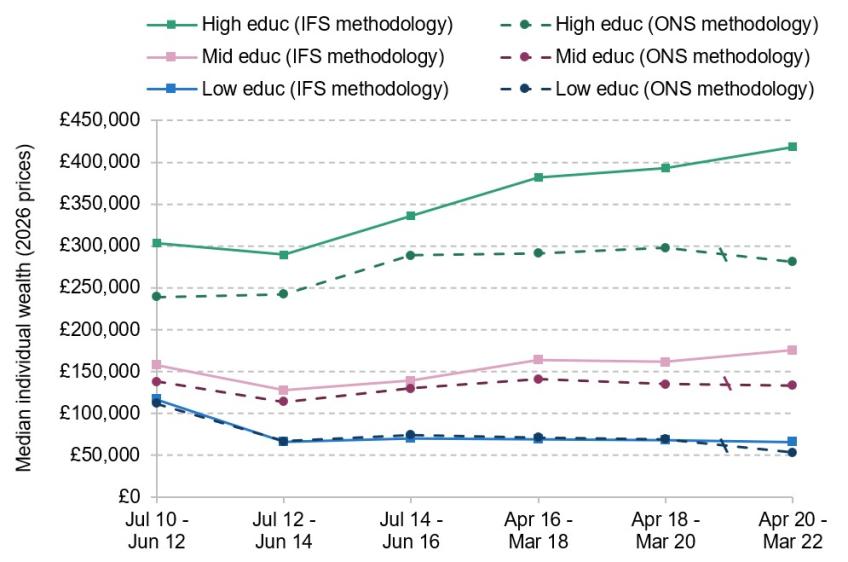
_{Note: High education refers to people who have a degree-level qualification or above. Mid education refers to people who have formal educational qualifications below degree level. Low education refers to people with no formal educational qualifications. The backward slashes show series breaks in the ONS methodology.}

_{Source: Authors’ calculations using Wealth and Assets Survey, Waves/Rounds 1–8.}

While our methodological changes alter the value of pension wealth, they do not do this uniformly for all individuals holding DB pensions (or pensions in payment). Rather, they imply a large increase in pension wealth for younger individuals, compared with much smaller increases, or even decreases, for older individuals (see Figure B3 in Appendix B). This is because the lower discount rate used to value future pension income in our methodology increases the current value of pensions most for the young, who will receive their pension income further in the future.27

Figure 7 shows explicitly how our methodology increases the importance of pensions for younger individuals. The figure sets out the composition of wealth holdings by age group under the ONS and IFS methodologies in 2020–22. While our methodology increases the share of measured wealth of the 65+ age group attributable to pensions from 31% to 38%, the impact is much greater for younger age groups. The 20–39 and 40–64 groups see pension wealth jump from comprising around 40% of total wealth for both groups to 59% for 40- to 64-year-olds and to 73% for 20- to 39-year-olds.

Figure 7. Composition of individual wealth by age group in the Wealth and Assets Survey Round 8 (April 2020 to March 2022)

_{Source: Authors’ calculations using Wealth and Assets Survey, Round 8.}

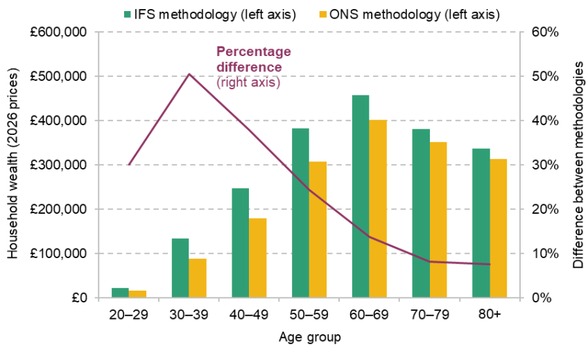
A direct result is that our improved measure of private pension wealth significantly alters the measured distribution of wealth by age. Figure 8 shows median individual wealth by age group under both methodologies in 2020–22. Apart from the youngest age group, who have accumulated very little wealth under either measure, there are larger percentage increases in wealth under our measure for younger individuals. Median wealth for individuals in their 30s is 50% higher under our measure than under the ONS measure; for individuals aged 70 and over, the increase is less than 10%. Even in cash terms, median wealth increases by more for individuals in their 30s than for individuals aged 70 and over, despite younger individuals having a much lower baseline level of wealth under the ONS methodology.

Figure 8. Median individual wealth in the Wealth and Assets Survey Round 8 (April 2020 to March 2022), by age and methodology

_{Source: Authors’ calculations using Wealth and Assets Survey, Round 8.}

This means that the share of total wealth held by younger individuals in 2020–22 was higher under our measure than under the ONS measure. Individuals aged 20–39 held 18% of aggregate wealth under our measure, compared with 11% under the ONS measure. At the same time, the share of wealth held by individuals aged 65 and over fell from 36% to 29% with our methodological changes.

The two measures also paint different pictures in terms of trends by age over time, as shown in Figure 9. Under the ONS methodology, the share of wealth held by individuals aged 65 and over increases steadily between 2010–12 and 2018–20 from 33% to 37%. Over the same period, the share held by individuals aged 20–39 remained essentially constant at 8%. In contrast, our methodology attributes a growing share of overall wealth to individuals aged 20–39 (from 10% in 2010–12 to 12% in 2018–20), and a much smaller increase in the share held by individuals aged 65 and over (from 30% in 2010–12 to 32% in 2018–20). In other words, when pension wealth is properly valued, the substantial shift in wealth towards those over the age of 65 previously recorded by WAS appears far more modest, while the share of wealth held by younger adults increased by more than previously thought.

Figure 9. Share of aggregate total wealth held by individuals of different ages

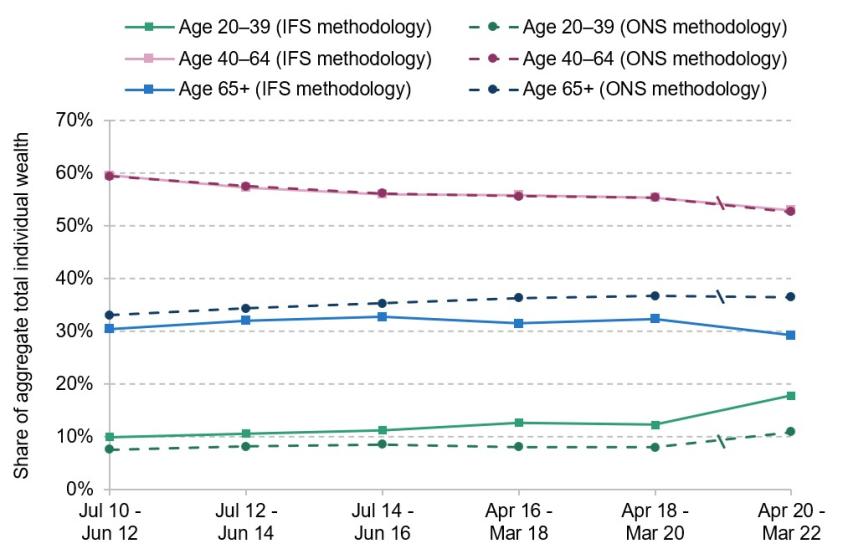
_{Note: We do not include individual wealth of people younger than 20 in the total wealth used in this figure so that the shares sum to 100%. The backward slashes show series break in the ONS methodology.}

_{Source: Authors’ calculations using Wealth and Assets Survey, Waves/Rounds 1–8.}

4. Conclusions

By any reasonable measure, retirement savings are one of the most important components of household wealth. However, it is challenging to assess the value of private pensions because they cannot be bought and sold. As this and previous work by IFS researchers (Adam et al., 2025) has set out, the current ONS approach to the valuation of pension assets in the Wealth and Assets Survey – the only comprehensive survey of the distribution of household wealth in Great Britain – is both flawed and inconsistent over time.

The methodology developed in this report seeks to begin the process of remedying that situation by developing a core methodology, based on sound economic principles, for the valuation of pension assets. Most importantly, it moves away from the use of the SCAPE rate, which is not appropriate for measuring the market value of pension promises, and towards the use of real UK government bond yields, which provide a reasonable measure of the risk-free interest rate.

Our hope is that this will serve both as a useful resource for future research28 and as a template for future improvements to official statistics. In the broadest terms, the principles that we highlight as crucial for the improvement of UK wealth statistics in the future are:

• Market value. The vast majority of non-pension wealth in WAS is measured on the basis of market value. In order to provide statistics that are capable of providing a meaningful measure of total household wealth, it is therefore crucial that pension wealth be measured on a similar basis. In practice, the key implication of this principle is that the basis for estimating pension wealth must be to discount future incomes using market interest rates.
• Updating past statistics. While resource constraints mean that the Office for National Statistics faces trade-offs about what it updates, there are real costs to making large methodological changes to datasets without applying that methodology to past years of the data. Were future improvements to be made to the ONS methodology, they should ideally be applied consistently over time.

Our improved approach has a significant impact on the estimated distribution of household wealth in the UK and how this has changed over time. Pension wealth made up a much higher share of household wealth in 2020–22 than suggested by official ONS estimates. Gaps in wealth by education were much wider than suggested by ONS, and had grown by more since 2010–12. Our methodology also increases the estimated share of wealth held by younger people and suggests that this share had increased since the early 2010s.

While we consider the methods described in this report to be a clear improvement on the status quo, we stress that our approach is far from the final word on how pension wealth is best to be valued for the purposes of household wealth statistics. As we discuss in Appendix A, knotty questions remain, not least how the tax treatment and illiquidity of pension assets should be reflected when undertaking valuation. How rich Britain’s households are is a less simple question than it might initially appear. But we hope that this report moves us closer to being able to provide the nation’s policymakers with a coherent answer to it.

Appendix A. Methodological approaches to valuing private pensions

This appendix provides a detailed account of the methodological approaches (both current and past) to the valuation of private pensions adopted by the Wealth and Assets Survey (WAS) and of the new ‘IFS methodology’ for the valuation of pension assets proposed in this report.

Current approach to pension valuation in the Wealth and Assets Survey

Here we provide a more detailed description than that provided in the main body of this report of the approach taken to the valuation of pensions in Round 8 of WAS (covering the period between April 2020 and March 2022), which at the time of writing is the most up-to-date version of the data available.

Pension schemes in the UK can generally be divided into two categories: defined benefit (DB) – including so-called ‘final salary’ schemes – and defined contribution (DC) – also known as ‘money-purchase’ schemes. DB schemes operate by providing members with a percentage of their final or career-average salary29 from a stipulated retirement age until death, with the percentage determined by the number of years that the individual was a member of the scheme during their working life. A DC pension differs from a DB pension in that it does not promise a particular level of pension income; rather, it is a fund into which contributions are paid and subsequently invested in a range of assets, with the value of the fund (and therefore the retirement income it can provide) depending on the amounts contributed and the investment returns achieved.

The method employed for valuing pensions in WAS differs both by whether the pension is a DB or DC scheme and by whether the respondent has begun receiving retirement benefits from the pension. For DC pensions from which no regular income is being drawn, the WAS approach to valuation is straightforward, with survey respondents simply asked the current amount of money saved in their pension pot. The valuation of DB pensions not yet in payment is more complex. WAS calculates the value of DB pension $i$ as follows:

  $PensionValu{e}_i=\frac{A_i{\alpha }_i{n}_i{s}_i+L_i}{(1+r{)}^{R-a}}$                                                                                 (1)

where

• $A_i$ is an ‘annuity factor’ specific to the sex, and normal retirement age ($R$), of the holder of DB pension $i$;30
• ${\alpha }_i$ is the ‘accrual fraction’ of DB pension $i$ (i.e. the additional percentage of the scheme member’s final or career-average salary that an additional year of membership in the scheme entitles the contributor to);
• $n_i$ is the number of years that the respondent has been a member of the scheme;
• $s_i$ is the respondent’s pre-tax salary at the time of interview;
• $L_i$ is any ‘lump-sum’ pension to which the individual is entitled as part of the scheme31
• $r$ is the discount rate;
• $a$ is the age of the respondent at the time of interview.

Intuitively, equation 1 attempts to take the total cash value at retirement of the stream of income that pension $i$ will yield in retirement, and converts it into today’s terms by ‘discounting’ over the period between the age at the time of interview and the age at which full pension benefits can begin to be drawn ($R-a$).

Pensions that are already providing the respondent with a regular income are valued in WAS using the same method regardless of whether the income is from a DB or DC scheme.32 For these schemes, the regular income that the pension provides is converted into a cash amount by means of an annuity factor:

$PensionValu{e}_i=A_{i}In{c}_i$                                                                                             (2)

where $A_i$ is a sex- and age-specific annuity factor (where the relevant age is the respondent’s age at the time of interview) and $In{c}_i$ is the regular amount of income provided by the pension. We discuss annuity factors in more detail in the next section.

Changes to the valuation of pensions in the Wealth and Assets Survey

The methodology described in the previous section has changed in a number of important ways since the publication of the first ‘wave’ of WAS (which covered the period July 2006 to June 2008). In this section, we summarise the most consequential of these changes.

The first major alteration in methodology occurred between Waves 2 (July 2008 to June 2010) and 3 (July 2010 to June 2012) of WAS. Two changes were made:

1. In Waves 1 and 2, the rate used to discount future DB pension incomes ($r$ in equation 1) was calculated based on real AA corporate bond yields as of 19 December 2009 and 17 December 2011 respectively. This resulted in a discount rate of 2.5% in Wave 1 and 1.8% in Wave 2 (Office for National Statistics, 2012). From Wave 3 onwards, WAS moved to setting $r$ equal to the Superannuation Contributions Adjusted for Past Experience (SCAPE) rate. SCAPE is a rate published by the government and designed to reflect the expected medium-term rate of nominal GDP growth.33 It was further decided that instead of using a single discount rate for all respondents, the discount rate would be set equal to the current level of the SCAPE rate in the month of interview.34
2. Annuity factors used in valuing pension assets ($A_i$ in equations 1 and 2) in Waves 1 and 2 reflected the second-best quoted RPI index-linked single-life annuity rates as quoted on 19 December 2009 and 17 December 2011 respectively. From Wave 3 onwards, annuity factors were changed to reflect the market price of annuities in the month of interview as opposed to at a single point in time for all respondents.

Taken together, these two changes resulted in a far lower estimate of aggregate pension wealth than was reached under the previous methodology. For example, when applied to the Wave 2 (2008–10) data, the updated methodology reduced the estimated aggregate level of retained DB pension wealth from £677 billion to £322 billion (Office for National Statistics, 2014). These methodological updates were retrospectively applied to Waves 1 and 2 of the survey, to avoid creating a structural break in the calculation of household wealth.

The second major change in methodology occurred between Rounds 7 (covering April 2018 to March 2020) and 8 (covering April 2020 to March 2022) of WAS. Four changes were made:

1. As described above, between Wave 3 and Round 7 of WAS (inclusive), the discount rate used in valuing DB pensions was the SCAPE rate. Unlike the AA-corporate-bond-based rate that preceded it, the SCAPE rate is a nominal and not a real discount rate. As shown by Adam et al. (2025), this methodology erroneously undervalued DB pensions by ignoring the fact that DB pension benefits are in almost all cases inflation-protected. In recognition of this, the discount rate used from Round 8 of WAS onwards is the real component of SCAPE (e.g. for SCAPE rate of CPI+1.7% in place from the end of March 2023, the discount rate would be set equal to 1.7%). This use of a real discount rate rather than a nominal discount rate is an improvement, though as explained in Section 2 of the main report, the use of the SCAPE rate is still an inappropriate way of measuring the value of DB pensions to individuals.
2. Up to and including Round 7 (2018–20) of WAS, annuity factors were determined by the market price of RPI index-linked single-life annuities. From Round 8 (2020–22) onwards, annuity factors are instead calculated directly by the Government Actuary’s Department (GAD). These annuity factors differ from the market rates used in previous vintages of WAS in a number of important ways:
   1. The GAD annuity factors are calculated on an actuarially ‘fair’ basis. In other words, they are set equal to the net present value of the income that an individual can expect to receive from an annuity which provides a regular income until death, given the expected longevity of the recipient. While market annuity rates follow a similar logic, their price will also reflect the costs to the insurer of providing the annuity and the characteristics (e.g. expected longevity) of those purchasing annuities.
   2. The discount rate used in discounting future annuity income is the real component of the SCAPE rate whereas market annuity rates implicitly embed market rates of interest for the purposes of discounting.
3. The GAD annuity factors are calculated on a ‘joint-life’ basis. This means that it is assumed that income will continue to be paid out to any surviving spouse or civil partner after the death of the scheme member.35 This differs from the previous approach where the market price chosen was for a ‘single-life’ annuity. The previous methodology made use of the market price for an RPI-linked annuity. While GAD continues to assume that the retirement income received from the pension being valued is inflation-linked, this is now indexed to CPI rather than RPI.
4. From Round 8 (2020–22) onwards, WAS imposes a blanket assumption that the holders of DB pensions are able to begin drawing their full pension no earlier than age 60 (this places a minimum value of 60 on the $R$ parameter of equation 1). This improves the previous state of affairs where a large number of individuals were treated as being able to start drawing their full pension implausibly early.36

The impact of this revision was extremely large, reducing the total estimated value of private pension wealth in Round 7 (2018–20) of the data from £6.4 trillion to £4.2 trillion (Office for National Statistics, 2024b). These changes were not applied retrospectively to previous editions of WAS data.

IFS pensions valuation methodology

In this section, we outline the methodology adopted in calculating a consistent set of pension values over time. Our starting point for producing a consistent methodology of pensions valuation is that used to produce the estimates in Round 8 of WAS. However, our approach differs in two ways:

• Discount rates. In equation 1, we set $r$ equal to the real gilt yield in the month of interview, with the maturity of the yield matched to the length of the period being discounted. This differs from the ONS methodology in Round 8 of WAS where $r$ is set equal to the real SCAPE rate. Our approach entails matching the yield maturity of the gilt to the number of years the respondent has before they reach their normal retirement age $R$. For example, for an individual aged 45 with a normal retirement age of 65, $r$ would be set equal to the expected real yield on a 20-year gilt. Real yields are derived by taking RPI-linked gilt yields from the Bank of England37 and reducing the yield to account for the 0.9 percentage point long-run difference between RPI and CPI inflation.38
• Annuity rates. As in Round 8 of WAS under the ONS methodology, we calculate annuity factors directly on an actuarially ‘fair’ basis based on ONS life tables.39 However, the discount rate underlying our calculation is again based on real gilt yields, whereas ONS uses the real component of the SCAPE rate in Round 8. To be specific, the formula for calculating actuarially fair annuity factors is as follows:

$A_i^{IFS}=\sum _{t=a}^{\infty }\frac{P_{it}}{(1+r_a{)}^{t-a}}$                                                                                  (3)

where $a$ is the age at which benefits begin to be received (set equal to normal retirement age $R$ for DB pensions not yet in payment or to the current age of the respondent for pensions in payment) and $t$ indexes all future years for which pension benefits will be received. $P_{it}$ is the probability that individual $i$ will survive to age $a+t$ given the sex and current age of the individual at the time of interview. As in the current Round 8 methodology, longevity is calculated on a joint-life basis.40 Estimates of longevity are sourced from ONS mortality rates estimates (Office for National Statistics, 2025). And $r_a$ is the discount rate, which is the principal difference between our approach and the ONS methodology. ONS uses the real component of the SCAPE rate as the discount rate in equation 3. We instead use the expected real yield on a gilt bought in the year the respondent reaches age $a$ with a maturity of 15 years as the discount rate.41

Outstanding issues regarding pension valuation in the Wealth and Assets Survey

While this report seeks to propose a more consistent and coherent approach to the valuation of pension assets in WAS, a number of concerns remain regarding how pensions are valued in the data that our improved approach does not currently address. In this section, we describe these outstanding concerns.

Tax treatment of private pensions

Private pensions are taxed differently from most other assets. Full income tax relief is available up front on the vast majority of pension contributions, and capital returns to investments made by pension funds are also tax-exempt. Instead, income tax is applied to pension withdrawals. If private pensions are to be valued in a way that is comparable to the market values used to value all other assets in WAS, these differences in tax treatment should in principle be taken into account. Evidently, for example, £1 on which income tax has yet to be paid is worth less than £1 on which income tax has already been paid.42 The kind of adjustment that would ideally need to be made to private pension values differs according to the type of pension under consideration:

• DB pensions and annuitised DC pensions. For these types of pensions, the only adjustment required is a reduction in value to account for deferred income tax due when funds are withdrawn from the pension.
• DC pension pots. As with DB pensions and annuities, values should be adjusted downwards to account for deferred income tax. For DC pension pots, however, a second adjustment is also required. This is to account for the fact that capital returns within pensions (e.g. in the form of dividends, interest and capital gains) are tax-exempt. All else equal, this fact makes assets held inside a pension relatively more valuable than the same assets held outside of a pension, and so would ideally require DC pension values to be adjusted upwards. The relative size of these adjustments will depend on a range of factors and could plausibly entail an overall adjustment that either increases or decreases the value of DC pension pots relative to our methodology.

While the principled case for such adjustments is strong, we do not include them in our estimates for two reasons. The first is that the magnitude of the adjustments described above is uncertain, particularly the adjustment for the tax exemption on capital returns.43 The second is that pensions are not the only kind of wealth where a principled case exists for making adjustments on the basis of tax treatment. For example, adjustment would ideally be made both to the value of assets held within individual savings accounts (ISAs) – which, like DC pensions, benefit from tax-free capital returns – and for latent capital gains tax liabilities associated with assets that have appreciated in value but not yet been sold.44 While some of these adjustments would be theoretically feasible in WAS, others (such as for unrealised capital gains) would not. As a result, we leave the issue of adjusting the value of assets to account for differences in tax treatment to future work.

Liquidity

Pension income generally cannot be accessed until an individual reaches their normal minimum pension age (currently 55 but set to rise to 57 in 2028). Furthermore, pensions cannot be used as collateral in taking out a loan. Were it possible to freely buy and sell pensions, this would significantly reduce their traded value. In other words, £100,000 in an accessible savings account is worth more than a £100,000 pension pot that cannot be accessed for many years. As in the case of tax treatment, it would be a fruitful (but far from straightforward) exercise to estimate the impact of this fact of pension wealth.

Annuitisation of DC pensions in payment

The use of the annuitisation procedure described in equation 2 for the valuation of DC pensions in payment raises two potential concerns. The first is that the value of the future income provided by the pension is assumed to remain constant in real terms. For DB pensions, where benefits are typically indexed to inflation, this is a reasonable assumption. Annuities purchased with DC pension pots, however, are generally not inflation-linked, meaning that the current methodology will tend to overvalue annuitised DC pension wealth.45 A further issue arises for individuals drawing a regular income from a DC pension in drawdown. In this case, annuitisation is not an ideal approach as pensions in drawdown do not offer a guaranteed lifetime income as annuities do.

Final versus average salary schemes

The method outlined in equation 1 provides a coherent means of valuing final salary DB pensions. It is increasingly common, however, for DB pensions to be calculated on the basis of members’ average salaries over the course of their careers. To accurately value such pensions would require setting $s_i$ equal to the career-average salary (rather than current salary) of the respondent. This is not currently information collected by WAS and all estimated DB pension values assume that schemes are based on the respondent’s final salary (likely resulting in an overestimate of the average value of DB pensions). This is going to become an increasing problem over time, as public sector workers accrue increasing fractions of their pensions under ‘career average’ scheme rules rather than ‘final salary’ rules.

Defined benefit lump-sum payments

Another area of concern relates to lump-sum payments ($L_i$ in equation 1). In order to ascertain the lump sum that will be received, the current WAS questionnaire asks: ‘What size lump sum do you expect to receive when you retire?’. This wording is flawed in a number of ways. First, there is a danger that respondents may reply to this question by telling the interviewer the lump sum that they expect to receive contingent on future contributions. This is inconsistent with the valuation exercise being conducted, which seeks to ascertain the value of an individual’s DB pension at the point of interview, not the future value of the pension after the respondent has made (potentially) many more years of contributions. In so far as respondents do provide an answer that is contingent on future contributions, this will tend to lead to an overestimate of the value of such lump sums.

Second, it is not clear whether the question is intended to elicit responses in nominal terms or real terms. As a result, it is likely that recorded responses contain some mixture of the two, making it difficult to know what the right approach is to discount the lump-sum component of pension wealth. Equation 1 will be correct only if respondents provide the value of the lump sum in real terms. In so far as respondents report $L_i$ in nominal terms, equation 1 will result in an overestimate of pension value. Third, many modern DB schemes do not offer an additional lump-sum component by default. Instead, they offer their members the option of taking a lump sum at retirement in return for a reduced pension income in subsequent years. This is the case in, for example, the public sector pensions now provided in the NHS, in the civil service and to teachers. If respondents are reporting lump sums of this kind, WAS will effectively introduce double counting: including the value of the lump sum without accounting for the reduction to subsequent pension income that this entails.

Misreporting of pension type

A final concern is that a significant number of respondents to WAS seem to misreport whether they have a DB or DC pension. Figure A1 illustrates this by showing the share of employees, by sector, who report currently saving into a DB or DC pension in WAS compared with employer-reported data (from the Annual Survey of Hours and Earnings, ASHE). While the overall share of employees who report saving in any type of pension closely matches the share in ASHE in both sectors, WAS does not appear to accurately capture the DB/DC split in either sector. This suggests that some people who are currently saving in a DB pension may report having a DC pension and vice versa. This raises concerns that we will inaccurately estimate their actual pension wealth. Future editions of WAS could help improve estimates of pension wealth by improving the clarity of the question intended to elicit whether a respondent’s pension is DB or DC, and introducing follow-up questions to people who report an atypical pension type for their sector.

Figure A1. Private pension participation rate split between defined benefit and defined contribution arrangements, in the Annual Survey of Hours and Earnings and the Wealth and Assets Survey, 2019

_{Source: Reproduced from figure A2 of Boileau, Cribb and Emmerson (2025).}

Appendix B. Additional figures

Figure B1. Mean household wealth over time by methodology 

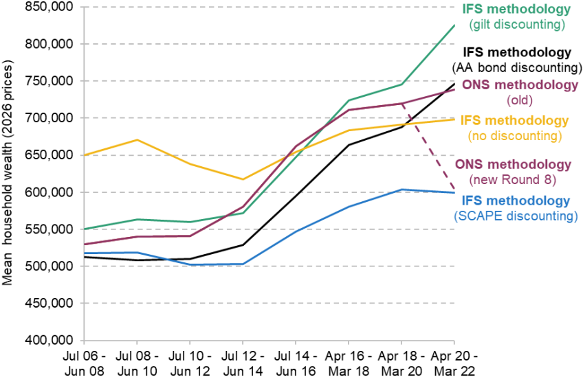
_{Note: Dashed line shows series break in ONS methodology.}

_{Source: Authors’ calculations using Wealth and Assets Survey, Waves/Rounds 1–8.}

Figure B2. Gini coefficient of household wealth over time by methodology

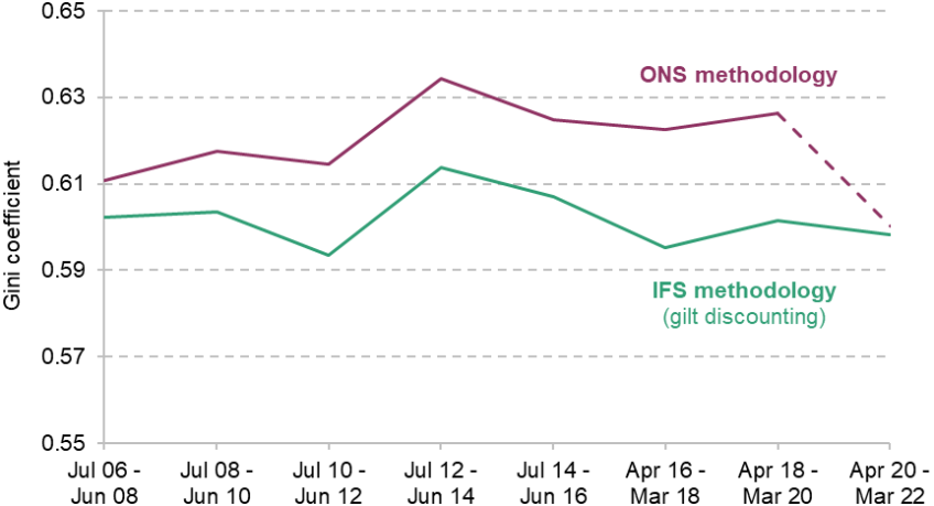
_{Note: Dashed line shows series break in ONS methodology. Households with negative wealth are not used to calculate Gini coefficient.}

_{Source: Authors’ calculations using Wealth and Assets Survey, Waves/Rounds 1–8.}

Figure B3. Ratio of total individual pension wealth calculated using IFS methodology (gilt discounting) versus total individual pension wealth calculated using ONS methodology by age group, over time

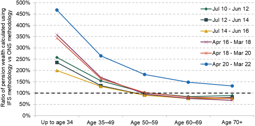
_{Note: We calculate total individual pension wealth by age group and data vintage both under the IFS methodology with gilt discounting and under the ONS methodology. This chart plots the ratio of these two measures by age group and time.}

_{Source: Authors’ calculations using Wealth and Assets Survey, Waves/Rounds 1–8.}

References

Adam, S., Delestre, I., Emmerson, C. and Sturrock, D., 2025. £2 trillion poorer than previously thought? Assessing changes to household wealth statistics. IFS Report, https://ifs.org.uk/publications/ps2-trillion-poorer-previously-thought-assessing-changes-household-wealth-statistics.

Advani, A., Bangham, G. and Leslie, J., 2021. The UK’s wealth distribution and characteristics of high-wealth households. Fiscal Studies, 42(3–4), 397–430, https://doi.org/10.1111/1475-5890.12286.

Boileau, B., Cribb, J. and Emmerson, C., 2025. Policies to help people manage defined contribution pension wealth through retirement. IFS Report, https://ifs.org.uk/publications/policies-help-people-manage-defined-contribution-pension-wealth-through-retirement.

Cochrane, J. H. (2005). Asset Pricing: Revised Edition. Princeton University Press.

Finkelstein, A. and Poterba, J., 2004. Adverse selection in insurance markets: policyholder evidence from the U.K. annuity market. Journal of Political Economy, 112(1), 183–208, https://doi.org/10.1086/379936.

Government Actuary’s Department, 2025. ONS Wealth and Assets Survey: pension wealth annuity factors – Round 8 guidance note. https://assets.publishing.service.gov.uk/media/685c1bef7d72089d19976141/ONS_Wealth_and_Assets_Survey_Pension_Wealth_Annuity_Factors_Round_8_Guidance_Note.pdf.

Karamcheva, N. and Perez-Zetune, V., 2023. Defined benefit and defined contribution plans and the distribution of family wealth. Congressional Budget Office Working Paper 2023-02, https://www.cbo.gov/publication/58305.

Krishnamurthy, A. and Vissing-Jorgensen, A., 2012. The aggregate demand for Treasury debt. Journal of Political Economy, 120(2), 233–67, https://doi.org/10.1086/666526.

Novy-Marx, R. and Rauh, J., 2011. Public pension promises: how big are they and what are they worth? Journal of Finance, 66(4), 1211–49, https://doi.org/10.1111/j.1540-6261.2011.01664.x.

Office for Budget Responsibility, 2024. Economic and fiscal outlook - October 2024. https://obr.uk/efo/economic-and-fiscal-outlook-october-2024/.

Office for Budget Responsibility, 2025. Economic and fiscal outlook – March 2025. https://obr.uk/efo/economic-and-fiscal-outlook-march-2025/.

Office for National Statistics, 2012. Annex on Pensions Wealth Methodology, 2008/10. Chapter 5 of Wealth in Great Britain Wave 2, 2008-2010 (Part 2), https://webarchive.nationalarchives.gov.uk/ukgwa/20160105200420/http://www.ons.gov.uk/ons/rel/was/wealth-in-great-britain-wave-2/2008-2010--part-2-/report--chapter-5--annex.html#tab-Discounting-and-financial-assumptions.

Office for National Statistics, 2014. Technical details. Chapter 7 of Wealth in Great Britain Wave 3, 2010-2012, https://webarchive.nationalarchives.gov.uk/ukgwa/20140723160245/http:/www.ons.gov.uk/ons/rel/was/wealth-in-great-britain-wave-3/2010-2012/report--chapter-7--technical-details.html#tab-Changes-to-the-estimates-of-private-pension-wealth-from-those-previously-published-from-the-Wealth-and-Assets-Survey.

Office for National Statistics, 2024a. Wealth and Assets Survey (WAS) Wave 5: validation of figures against external sources. https://www.ons.gov.uk/peoplepopulationandcommunity/personalandhouseholdfinances/incomeandwealth/methodologies/wealthandassetssurveywaswave5validationoffiguresagainstexternalsources.

Office for National Statistics, 2024b. Estimating defined benefit pension wealth in Great Britain: December 2024. https://www.ons.gov.uk/peoplepopulationandcommunity/personalandhouseholdfinances/incomeandwealth/articles/estimatingdefinedbenefitpensionwealthingreatbritain/december2024.

Office for National Statistics, 2025. Past and projected mortality rates (qₓ) from the 2022-based Great Britain life tables. https://www.ons.gov.uk/peoplepopulationandcommunity/birthsdeathsandmarriages/lifeexpectancies/datasets/mortalityratesqxprincipalprojectiongreatbritain.

Poterba, J., 2004. Valuing assets in retirement saving accounts. National Tax Journal, 62(2), 489–512, https://doi.org/10.17310/ntj.2004.2S.06.

UK Data Service, undated. Household Assets Survey Round 8 Main-Stage Questionnaire. UK Data Archive Study Number 7215 – Wealth and Assets Survey, https://doc.ukdataservice.ac.uk/doc/7215/mrdoc/pdf/7215_was_questionnaire_round_8_covid19_version.pdf.

van Binsbergen, J. H., Diamond, W. F. and Grotteria, M., 2022. Risk-free interest rates. Journal of Financial Economics, 143(1), 1–29, https://doi.org/10.1016/j.jfineco.2021.06.012.

Data

Office for National Statistics, Social Survey Division. (2025). Wealth and Assets Survey, Waves 1-5 and Rounds 5-8, 2006-2022. [data collection]. 20th Edition. UK Data Service. SN: 7215, DOI: http://doi.org/10.5255/UKDA-SN-7215-20.

Acknowledgements

The authors gratefully acknowledge the support of the ESRC Centre for the Microeconomic Analysis of Public Policy (ES/Z504634/1). They are grateful for advice and comments on this work from Stuart Adam, Jonathan Cribb, Carl Emmerson, Chris Giles and David Sturrock. This work was produced using statistical data from the Wealth and Assets Survey, produced by the Office for National Statistics. Data from the Wealth and Assets Survey are Crown Copyright and are reproduced with the permission of the Controller of HMSO and the King’s Printer for Scotland.