New estimates of the impact of undergraduate degrees on lifetime earnings

Executive summary

What is the effect of going to university on earnings over graduates’ lifetimes? To what extent do subject choice, institution and the prior academic attainment of those students matter? How much do individuals (and taxpayers) benefit from people going to university, once we account for the costs of financing higher education, and the tax and student loans systems? With around half of young people in England now entering university, evidence on these questions is as important as ever – both for individuals deciding whether, where and what to study, and for policymakers concerned with financing higher education.

This report investigates the lifetime financial returns to starting a full-time undergraduate degree at a UK university before age 21. We use detailed data on a cohort of England-domiciled students who were born in the mid 1980s and took their GCSE exams in 2002. We estimate how much graduates from this cohort can expect to earn over their lifetimes, and also how much they would have earned over their lifetimes had they not gone to university. We use these estimated gross lifetime returns for the 2002 GCSE cohort as an estimate of the gross returns that can be expected by future cohorts; available evidence supports this choice. We apply today’s tuition fee, student loan and tax policies to consider how these returns, net of the costs of a degree, would be shared between graduates themselves (through higher take-home pay) and the government (through student loan write-offs and higher tax revenues) under current policy. We produce estimates of the lifetime return to degrees that are informative for current and prospective students and policymakers.

This is the latest in a series of reports by researchers at the Institute for Fiscal Studies, commissioned by the Department for Education, using the Longitudinal Education Outcomes (LEO) data, which link school records, university records and tax data for English students. The work follows on from Britton et al. (2020), who also estimated the lifetime returns to higher education (HE) for the same 2002 GCSE cohort based on their observed earnings to age 30, which is relatively early in people’s careers. This report updates and extends that evidence base, drawing on seven additional years of tax data (up to 2023/24) that allow us to observe how the earnings of the same set of graduates actually evolved into their mid 30s.

This work focuses on the financial returns to higher education: the earnings benefit for individuals over working life and the tax benefits for government net of the cost of financing higher education. It does not seek to provide a complete picture of the impacts of higher education – for instance, on pension contributions, health, happiness or job satisfaction, or potential spillovers to others. We study the returns to undergraduate degrees for students who actually enrolled in them. Our results should not be interpreted as the returns that would be realised if the higher education sector were significantly expanded or contracted, or if large numbers of students were reallocated across courses and universities.

1. Introduction

Higher education has expanded dramatically in England over recent decades, with around half of young people now entering university.1 This expansion has been underpinned by a system for financing higher education that shifts a significant share of the costs of degrees onto graduates themselves in the longer run, while aiming to protect graduates who go on to have low earnings after university from unaffordable student loan repayments. Against this backdrop, understanding the financial returns to higher education – who gains, by how much, and whether those gains justify the cost to both individuals and the taxpayer – is a central question for higher education policy. This report investigates the lifetime financial returns to starting a full-time undergraduate degree at a UK university before age 21.

Previous work at IFS (Britton et al., 2020) has documented large average returns to individuals attending university, but also striking variation: returns differ enormously by subject studied and by institution, and some graduates see little or no financial benefit from their degree. However, those estimates were based on individuals tracked only up to age 30 in the labour market, which is relatively early in people’s careers, and used data up to the 2016/17 tax year. This report updates and extends that evidence base, drawing on seven additional years of tax data (up to 2023/24) that allow us to observe how the earnings of the same set of graduates actually evolved into their mid 30s.

Our approach involves linking individuals’ school, university and tax records so we can observe their background characteristics (gender, ethnicity and socio-economic background), their attainment in Year 6 SATs, GCSEs and A levels, the university they attended and the subject they studied, and their earnings. We focus on a cohort of England-domiciled students who were born in the mid 1980s and took their GCSE exams in 2002. We observe how much they earn in each tax year up to age 37 and, beyond this age, we simulate their employment and earnings over the rest of their working lives. These simulations reflect historical patterns of earnings growth and employment transitions at later ages, and are based on some additional administrative data and the Labour Force Survey. We predict counterfactual employment and earnings profiles for the 2002 GCSE cohort if they had not attended higher education. Comparing this with their actual (and simulated) earnings allows us to estimate the gross lifetime earnings return to a degree.

We then apply today’s tuition fee, student loan and tax policies, to approximate the policies that would apply for someone aged 18 in 2025/26. We do this to make our results as relevant as possible for current students and policymakers. This allows us to estimate how the financial return to higher education – and the cost of a degree – would be split into a net return to the individual (through higher take-home pay) and a net return to the exchequer (through student loan write-offs and higher tax revenues) under current government policy. The results of this accounting exercise can be interpreted as the net returns to undergraduate degrees for the 2002 cohort, had they instead faced today’s policies (and assuming that their earnings would not have themselves been influenced by the policies in place).

We describe the data we use (Chapter 2) and our methodology (Chapter 3) which closely follows that in Britton et al. (2020). We describe the actual earnings of graduates and non-graduates from the 2002 GCSE cohort (Chapter 4). We then estimate individual and exchequer lifetime returns for those who attend higher education under current government policy, and investigate how these vary by gender, subject and institution type (Chapter 5). We discuss the conceptual limitations of our approach, including what these estimates can and cannot tell us about policy, and then assess how sensitive our main estimates are to alternative modelling decisions (Chapter 6). We compare our new headline estimates with those from previous work at IFS and explore why our estimates have changed (Chapter 7). We then investigate the returns for students with relatively low prior attainment (Chapter 8). Finally, we consider how useful our estimates of lifetime returns may be for later cohorts of students, adding new evidence to the important question of how the graduate premium may have been changing over time (Chapter 9).

2. Data

We use the Longitudinal Education Outcomes (LEO) dataset, which links labour market outcomes to school, further education and higher education records. We specifically use:

• school attainment records and demographic characteristics from the National Pupil Database (NPD);
• university records from the Higher Education Statistics Agency (HESA);
• earnings and employment data from HM Revenue & Customs (HMRC).

The NPD records contain rich background characteristics, including a student’s ethnicity, their home region and their eligibility for free school meals. They also contain rich details on a student’s prior attainment, including their scores in standardised tests at age 11 (Year 6 SATs) and their subject choices and scores for both GCSE and A-level exams. The HESA records track students through the university system, detailing the subject and institution for all courses taken by the student. The HMRC records contain data on annual earnings between tax years 2003/04 and 2023/24. From 2013/14 onwards, this includes income from self-employment from self-assessment tax records. Prior to this, we only observe earnings from employment.

The earliest cohort for which we have this fully linked administrative data took their GCSEs in the 2001/02 academic year, and the vast majority of them were born in 1985/86. We focus on this cohort for our main analysis (hereafter referred to as the ‘2002 GCSE cohort’). Among the students for whom we have rich information on background characteristics from school records, this is the cohort for which we can observe earnings at the oldest age. We observe earnings for this cohort between ages 17 and 37.

We also use the Labour Force Survey (LFS), a quarterly survey of approximately 40,000 UK households. Survey questions include demographic details, educational qualifications including subject studied at university, employment and earnings. Households are surveyed for five consecutive quarters and are asked questions on earnings in the first and final waves. We derive two datasets from the LFS: first, a five-quarterly LFS panel, linking individuals’ responses from waves 1 and 5, which we use to examine year-on-year changes in employment and earnings for individuals who respond to both waves; and second, a repeated cross-section of earnings, a snapshot of employment and earnings each quarter for a larger sample of individuals. We use both the year-on-year changes and the repeated cross-section to simulate earnings and employment transitions beyond age 37 for our cohort of interest. We use LFS data from 1997 up to March 2020.2 

For graduates, we also complement our simulations using additional administrative data: linked HESA and HMRC records for students from the 1978/79 to 1984/85 birth cohorts. For these students, we observe degree subject and institution attended, but none of the data on demographic characteristics or prior attainment that we take from school records for later cohorts. We observe earnings and employment for these students up to age 44 at the latest and use these data to simulate earnings trajectories for graduates in our cohort of interest between the ages of 38 and 44.

2.1 Sample selection

We restrict our main analysis sample to individuals from the 2002 GCSE cohort who achieved at least the points equivalent of five C grades in their top eight GCSE exams. We also require individuals to have a Key Stage 5 record within three years of the year in which they sat their GCSEs. We apply these criteria to ensure that our analysis is limited to people who could have chosen to enter university at, or soon after, age 18.

Following Britton et al. (2020), we focus on the returns to a specific ‘typical’ higher education (HE) trajectory: full-time undergraduate study beginning between the ages of 17 and 21. We exclude those who we observe to start a first undergraduate degree after age 21 or who studied part-time. We also exclude those who have only attended university for an ‘other undergraduate degree’ such as a foundation degree, unless they go on to begin a first undergraduate degree by age 21. We exclude these groups because their returns are likely to differ substantially, and constructing a credible counterfactual is considerably more challenging. Our comparison is therefore between students attending university for a full-time first undergraduate degree and individuals not attending university at all.3 We refer to these as the HE and non-HE groups hereafter for brevity, notwithstanding that in other contexts HE often refers to all study at Level 4 or higher.

Finally, note that we include all those who start a given course in our HE group, regardless of whether they are observed to graduate or to later switch course. This means we are considering the returns to attending university for an undergraduate degree, rather than completing a degree (we use the terms ‘graduates’ and ‘non-graduates’ for our HE and non-HE groups for ease of exposition, even though some individuals in our HE group do not graduate).

Altogether, our main analysis sample consists of 209,131 individuals, of whom 158,224 (76%) are in our HE group and 50,907 are in our non-HE group. More details on sample selection and sample sizes by sex and institution type are given in Appendix A.

3. Methodology

There are two substantial methodological challenges in estimating the lifetime returns to higher education (HE). First, data limitations mean that we are not able to observe people over the entire life cycle. This limitation is structural: even if we could observe a cohort that had completed their time in the labour market (born in the early 1950s, say), their returns to higher education would not be especially relevant to today’s graduates. Second, people self-select into different HE pathways. This means those who do and do not attend HE may differ in important ways, and they may have different earnings trajectories for reasons other than that some attended university and some did not.

Our approach closely follows Britton et al. (2020). We address these challenges by using data on the 1985/86 birth cohort – the oldest cohort for which we observe detailed background characteristics, which are crucial for addressing the self-selection issue. This cohort is sufficiently recent to still be informative as to the returns to HE today, but is old enough that we observe sufficient years of earnings to estimate lifetime returns. We are now able to observe this cohort’s earnings up to age 37 and then we simulate their employment and earnings up to age 67.

Our method for the simulation combines information on the levels and dynamics of earnings and employment from older graduates and non-graduates in their mid and late careers with long-run official forecasts of economy-wide real earnings growth. For data on older cohorts, we mainly rely on the Labour Force Survey (LFS), but also on some linked administrative records of people who attended university in the mid 1990s. We describe the simulation process in more detail in Section 3.1. The results of these simulations for our HE and non-HE groups are presented in Chapter 4.

Once we have actual (and simulated) earnings paths to retirement for both those who do and those who do not attend HE, we then fit econometric models to estimate the returns to attending HE at each age. This relies on comparing the earnings of individuals who attended HE with those who have similar observable characteristics in the Longitudinal Education Outcomes (LEO) data but who did not attend HE. We use these estimated returns to generate counterfactual earnings profiles for those who attended HE, predicting what they would have otherwise earned if they had not attended HE. The difference between the HE (actual and simulated) and the counterfactual earnings paths provides an estimate of gross earnings returns at each age and for each individual in the 2002 GCSE cohort. We sum these over the lifetime to calculate an individual’s gross lifetime earnings returns.

To make our results as relevant as possible for current students and policymakers, we then apply today’s tuition fee, student loan and tax policies to these gross lifetime earnings returns, approximating the policies that would apply for someone aged 18 in 2025/26. This allows us to estimate how the financial return to higher education – and the cost of a degree – would be split into a net individual lifetime return (through higher take-home pay) and a net return to the exchequer (through student loan write-offs and higher tax revenues) under current government policy. We discuss our approach for estimating returns further in Section 3.2 and we present results in Chapter 5.

Our approach for constructing counterfactual earnings at each age draws upon the rich background information from the National Pupil Database (NPD), which includes information about students’ socio-economic background, demographic characteristics (such as gender and ethnicity) and detailed information on attainment during primary and secondary school. While controlling for these characteristics is a substantial improvement on comparisons of average earnings of graduates and non-graduates, or of those studying different subjects, it is still unlikely to recover the true causal effect of attending HE. In particular, there may be student selection into attending HE based on characteristics that we do not observe in the LEO data and therefore cannot control for, but which have some independent relationship with future earnings: in other words, there may be selection on unobservables. It is typically assumed that a rich selection on observables approach such as ours will somewhat overstate the true causal returns to HE, although this is not certain. We discuss these and other limitations in detail in Chapter 6, as well as describing how robust our main estimates are to different modelling approaches.

We also extend the work of Britton et al. (2020) in two further ways. First, we consider the lifetime returns to HE separately by prior attainment (Chapter 8). Given the dramatic expansion in the number of young people attending university in England over recent decades, the returns for students with lower prior attainment (who are closer to being ‘academically marginal’) are of particular interest. Second, we draw on additional years of tax data to investigate how returns have changed over time for later cohorts of students, and on the latest student entrant data to suggest how changes in the composition of students might have affected average returns (Chapter 9). We describe our approach to the analysis underlying the results in these chapters in Sections 3.3 and 3.4 respectively.

3.1 Modelling life-cycle earnings

We observe earnings and employment for the LEO sample up to age 37 and simulate their labour market outcomes between ages 38 and 67.

Transitions at adjacent ages in the labour market are at the heart of our simulations of life-cycle earnings. We model each individual’s labour market outcomes at a given age as a function of their employment status and income rank within their cohort at the previous age. Our models are estimated on labour market transitions in the LFS and are then applied to the 2002 LEO sample to project forwards from age 37 up to retirement at age 67.

Our focus on transitions captures two important features of life-cycle earnings. First, an individual’s earnings usually do not change smoothly as they age. Instead, they may move between employment and unemployment and experience discrete jumps and falls in their earnings. This is especially important when estimating life-cycle returns net of taxes and student loans, as the tax and loan systems are non-linear. Second, earnings are correlated over time: relatively high earners at a given age are likely to be high earners at the next age. Our model reflects this persistence at adjacent ages, while allowing for potential earnings and employment shocks each year.

We allow the models to vary by sex and by subject studied at university. Given sample constraints in the LFS, we are unable to estimate separate labour market transitions for each university subject; instead, we split the sample into four groups and estimate separately by sex within each group. Following Walker and Zhu (2013) and Britton et al. (2020), these groups are those studying STEM subjects (science, technology, engineering and maths), those studying LEM subjects (law, economics and management), those studying other degree subjects and non-graduates.

Simulating employment

We model employment at each age and for each individual as a function of the individual’s employment status at the previous age and, if they were employed, their earnings rank at the previous age.4 

For those employed at the previous age, we predict the likelihood of an individual remaining employed as a function of their earnings rank at the previous age, using a probit model. This is estimated using the five-quarterly LFS panel data, separately by sex and subject group. For those unemployed at the previous age, we do not observe an earnings rank and so instead assume their probability of being employed at an age matches the mean rate of employment amongst people of the same age and in the same sex–subject group in the LFS who were unemployed at the previous age.5 

We have different definitions of employment in the administrative and survey data, and these also cover different time periods. To avoid jumps in the estimated employment rate between the ages of 37 and 38, we adjust the parameters estimated in the survey data so that they are consistent with the parameters we would have estimated from applying the same method to the administrative data at an overlapping age. This is done by fitting an identical model to the administrative data at the age 36–37 transition, saving the ratio of the parameters estimated using the administrative and survey data, and adjusting the parameters estimated at each later age in the survey data by this same ratio.

Using the fitted, smoothed and adjusted parameters, we calculate a probability of each individual in the LEO sample being employed at a given age, given their earnings rank in the previous year, and we randomly assign their employment status accordingly. We do this iteratively for all transitions from 37–38 up to 66–67.

Simulating earnings rank

Similarly, we model earnings rank at each age and for each individual as a function of the individual’s earnings rank at the previous age. We use a copula method to capture intertemporal dependence in earnings ranks.6 Given an individual’s position in the earnings distribution at the previous age, a copula function describes the probability distribution of that same individual’s earnings rank at the next age. Intuitively, this method allows us to capture that an individual’s earnings rank strongly but not perfectly predicts their earnings rank the following year, so that there is some re-ranking between ages.

We estimate copulas from the five-quarterly LFS data, separately by age, sex and subject group. As with modelling employment, we adjust the parameters to account for differences between the administrative and survey data. We use the estimated copula parameters to simulate a rank in the earnings distribution for each individual in our sample at each age, given their earnings rank in the previous period, beyond age 37. For those unemployed at the previous age, we cannot use the copulas to simulate a rank. Instead, we retain the earnings ranks of individuals of the same age, sex and subject group who re-enter employment in the LFS and randomly assign one of these ranks to individuals re-entering employment in our sample. We do this iteratively for all transitions from 37–38 up to 66–67.

Assigning earnings levels to ranks

Having assigned individuals at each age a rank in the earnings distribution (amongst people of the same age, sex and subject), we then need to assign actual earnings levels to these individuals, if they are employed in our simulation. To do this, we need to model how earnings will change for a set of individuals at consecutive ages. For this exercise, we do not rely on individual labour market transitions (i.e. repeated observations of earnings for the same individual over time) but instead use cross-sectional data on all individuals observed at a given age. This means we can use individuals reporting their earnings in only one wave of the LFS, increasing our sample size. Using this larger sample, we can estimate profiles of earnings growth over age separately by sex and for each subject, rather than by subject group.

Additionally, we use linked HESA–HMRC data for cohorts of students that are slightly older than our 2002 GCSE cohort. The samples by subject and age are much larger and more recent in these administrative data, so we favour the HESA–HMRC data over the LFS where possible. These data are not available for our non-HE group as only those who attend higher education have a HESA record. For our HE group only, we use HESA–HMRC cohorts born between academic years 1978/79 and 1984/85 to construct earnings profiles up to age 44, then use the LFS to extend these profiles beyond age 44, as shown in Figure 3.1.7 In Chapter 6, we also show the robustness of our results to using the LFS only for ages 38 to 44 instead of the HESA–HMRC data.

Figure 3.1. Schematic representation of our methodology

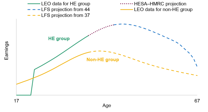
_{Note: The figure provides a schematic representation of the actual and simulated earnings for individuals from our HE and non-HE groups.}

Extracting measures of earnings growth by age from observational data is challenging because each birth cohort is only observed at a given age in a single period. For instance, if 38-year-olds are observed to earn more than 37-year-olds in a given year, this could be because the 38-year-olds have an extra year of experience (an age effect) or might reflect something about the specific cohorts – for instance, that the 37-year-olds initially joined the labour market during a recession or had different experiences at school (a cohort effect). Equally, if individuals in the same cohort (who were in the same school year) are observed to earn more in 2025 than they did in 2024, this could reflect an age effect, or economy-wide earnings growth between 2024 and 2025 (a period effect). It is in general impossible to disentangle the effect of changes in age from changes in period and cohort without making substantive assumptions. In the economics literature, this difficulty is known as the age–period–cohort problem.

Our preferred approach to this problem is to take a ‘simple period view’: we effectively assume that there are no cohort effects, and attribute earnings differences across cohorts in a given year to age effects rather than to cohort effects.8 More specifically, we de-mean earnings data from the LFS or HESA–HMRC data within tax years, removing variation in average earnings over time that is due to changing macroeconomic conditions. We then compare de-meaned (log) earnings at each pair of adjacent ages, and perform this exercise separately by sex and subject: intuitively, we pool across many years of data and, for example, compare the earnings of women aged 40 who studied law with the earnings of women age 41 who studied law, to estimate how the earnings of women who studied law typically change between these ages.9 This is only one possible way of extracting measures of earnings growth with age from data on previous cohorts. We discuss several alternative methods, and the robustness of our results to these, in Chapter 6 and Appendix G.

For non-graduates, we calculate average (log) earnings growth at each percentile of the earnings distribution, separately by age and sex, and apply these earnings growth rates to each percentile of the distribution of non-graduate earnings observed in the LEO data at age 37. This allows us to simulate a full distribution of non-graduate earnings at each later age. For our HE sample, we also start with the earnings distribution observed in administrative data by sex and subject, but then adjust the mean and standard deviation of the earnings distribution by sex and subject group at each later age based on by-age changes observed in the LFS. We sample systematically from the resulting distribution to map specific earnings levels at each age onto earnings ranks.

We must also account for how economy-wide earnings might change over time in future years, independent of age effects. To do so, we apply forecast long-run real growth in average weekly earnings based on the latest published official forecasts from the Office for Budget Responsibility (OBR), which currently project real growth of 1.8% each year in the long run.10 In Chapter 6, we show the sensitivity of our results to a less optimistic real earnings growth projection. Importantly, the projection used affects the simulated levels of both graduate and non-graduate earnings, but also implicitly changes how important earnings differences are at later ages compared with at earlier ages.

Modelling retirement

Changing retirement patterns over time are a threat to the reliability of our life-cycle simulations. This is especially true for women, where the state pension age for some women we observe in the LFS data was 60. It has since risen to 66 and is soon set to increase to 67. To reflect rising retirement ages in later cohorts relative to those observed at older ages in the LFS data, we fix model parameters for eight years at age 51, with parameters from ages 60 to 67 corresponding to ages 52 to 59 in the data. In practice, our estimated returns will not be dramatically affected by what happens to employment rates of individuals later in life as earnings are discounted; earnings towards the end of people’s working lives will have a smaller impact on their total discounted lifetime earnings than earnings at the start of their careers. We show the impact of an alternative approach to modelling retirement in Chapter 6.

3.2 Estimating returns

As described above, a key challenge is addressing the self-selection problem. Those who attend university tend to have performed better at school and on average come from higher socio-economic status backgrounds. The NPD data allow us to adjust for a very rich set of prior attainment and background characteristics that are likely to be correlated with both an individual’s choice to attend higher education and their labour market outcomes. We do this in a regression model which we use to develop a counterfactual gross earnings profile for each graduate had they not attended HE. We then calculate net (post-tax) earnings by applying the tax and student loan systems. We approximate net individual lifetime returns based on the difference between net graduate earnings (using actual data up to 37 and simulated data thereafter) and net counterfactual earnings.

Assigning counterfactual employment

We assign a counterfactual employment status for every graduate had they not attended HE. This is important because whether someone attends university will also have an effect on the probability of them having positive earnings in any given year.

We estimate a probit model for the probability of being employed at a given age as a function of a set of background characteristics observed in school records – specifically,

• scores in maths, English and science in Year 6 SATs (Key Stage 2 exams taken at age 11);
• scores in maths and English GCSEs and overall points score in GCSEs (Key Stage 4 exams typically taken at age 16);
• UCAS points obtained in Key Stage 5 exams;
• dummies for whether an individual studied maths, sciences, social sciences, arts, humanities, languages, vocational or other subjects at Key Stage 5;
• dummies for the region in which students were living in the year they took GCSE exams;
• dummies for nine different ethnic groups (e.g. White, Black African, Black Caribbean);
• various proxies for a student’s socio-economic status, measured in the year they took GCSE exams – specifically, whether they were eligible for free school meals, the Income Deprivation Affecting Children Index (IDACI) quintile of the small area in which they lived and whether they were attending a private school;
• whether they were recorded as having special educational needs;
• whether or not English was their first language.

We estimate this model on our sample of non-graduates, separately by sex and age, and use the fitted models to estimate a counterfactual employment rate amongst those who studied each subject, by sex and age. Each graduate begins with their actual (or simulated) employment at each age, and we then randomly assign additional graduates to be employed (or unemployed) in their counterfactual scenario to match these counterfactual employment rates by sex, age and subject.11 Intuitively, we reflect that both an individual’s actual employment status in the LEO data and their observable characteristics – which predict employment amongst non-graduates – are informative as to the probability that individuals in our HE group would have been employed had they not attended university.12 

Estimating counterfactual earnings and gross earnings returns

To construct counterfactual earnings, we estimate the following regression at each age, separately by sex:

$\log y_{i,a}={\delta }_a+{(Subjec{t}_i\times HEItyp{e}_i)}^{\text{'}}{\beta }_a+x_i^{\text{'}}{\gamma }_{1a}+H{E}_i{x}_i^{\text{'}}{\gamma }_{2a}+e_{i,a}$   (3.1)

where $\log y_{i,a}$ is the log of individual i’s income at age a, $Subjec{t}_i\times HEItyp{e}_i$ are dummies containing the interaction terms between our 31 subject classifications and 4 institution type categories, and $x_i^{\prime }$ is a set of background characteristics – the same set as in the bulleted list above. We allow the effect of all these background characteristics to vary between graduates and non-graduates by interacting them with a dummy for whether an individual attended higher education (denoted $H{E}_i$). Finally, ${\delta }_a$ accounts for varying levels of earnings at each age, and $e_{i,a}$ is an idiosyncratic error term.

Between ages 38 and 67, we fix the coefficients on our control variables at their age-37 values. The assumption here is that in relative (log) terms, the effect of background characteristics will be roughly constant across the life cycle from age 37. This assumption is necessary because, from age 37 onwards, we are relying on simulated earnings that are unlikely to completely capture dependence on background conditions. For example, this allows us to reflect that among individuals with identical earnings at age 37 who studied the same subject at the same university, those who performed better at school may still have higher future earnings expectations than those who did not perform as well.

The regression coefficients provide a predicted return for each individual graduate at each age, which is the effect of their $Subjec{t}_i\times HEItyp{e}_i$ interaction, combined with the differential effect of their individual background characteristics for graduates:

${\hat{r}}_{i,a}={(Subjec{t}_i\times HEItyp{e}_i)}^{\text{'}}{\hat{\beta }}_a+H{E}_i{x}_i^{\text{'}}{\hat{\gamma }}_{2a}$

As above, for ages 38 to 67 we fix the coefficients on the control variables at their age-37 values. We then subtract this predicted return from graduates’ earnings to generate their counterfactual earnings:

$y_{i,a}^{*}=\exp (\log y_{i,a}-{\hat{r}}_{i,a})$

This calculation only applies to those with positive actual (or simulated) earnings. For those who do not have positive actual earnings but who are employed in the counterfactual scenario, we assign counterfactual earnings by setting the $Subjec{t}_{\mathit{i}}$, $HEItyp{e}_i$ and $H{E}_{\mathit{i}}$ variables to 0 and predicting their earnings based only on their background characteristics, $y_{i,a}^{*}=\exp \left(\log {\hat{y}}_{i,a}^{*}\right)$.

This set-up enables us to estimate gross earnings returns separately by subject and institution type, for each gender.

Estimating net individual and exchequer returns

To move from gross earnings returns to estimates of net individual (and exchequer) returns, we apply the tax and student loan systems to the actual (and simulated) and counterfactual earnings of our HE group each tax year. We model these systems as if the cohort we study were 18 years old in the 2025/26 academic year to make our results as relevant as possible for policymakers and for those beginning undergraduate degrees now. In order to capture real earnings growth between the two cohorts, we adjust the earnings of the 2002 GCSE cohort in line with real earnings growth for the whole economy in the period between 2004/05 and 2025/26, when the respective cohorts would be at or entering university. This adds around 5.4% to all graduate and non-graduate earnings at all ages.13 

We then apply the income tax, employee National Insurance and employer National Insurance rates and thresholds that applied in the 2025/26 tax year and project thresholds forwards in line with current government policy. For instance, this means we model planned cash-terms freezes in personal income tax thresholds until April 2031, after which point we assume these thresholds will rise each year in line with forecast CPI inflation.14 To make the modelling manageable, we do not differentiate between employment and self-employment earnings even though these are taxed differently.

We estimate student loan borrowing, assuming students borrow the maximum they are entitled to for both tuition fees and living costs. The amount we estimate individual students borrow reflects how many years they study for, their socio-economic background and whether they study at a university in London. We estimate average borrowing of £52,000 in today’s prices amongst those who borrow for three years of study. This roughly matches the latest published DfE forecasts for average loan borrowing of £49,300 amongst full-time HE students who started courses in 2025/26 and took out three years of loans (Department for Education, 2025a). We model student loan repayments over the life cycle assuming that students face the ‘Plan 5’ student loan terms available to undergraduate students starting courses in 2025/26. In Chapter 6, we show the sensitivity of our results to instead applying the terms of ‘Plan 2’ student loans, which were available to those who started courses between 2012/13 and 2022/23. Further technical details on how we estimate student loan outlay and repayments are provided in Appendix B.

While the vast majority of up-front spending on HE is now in the form of government-backed loans, we also estimate government spending on grants to universities for teaching particular courses. This high-cost subject funding accounts for around 70% of recurrent funding that the Office for Students distributes.

Converting earnings streams into lifetime estimates

To compare costs and benefits stretching over many years in ‘present value’ terms, we convert earnings streams into ‘lifetime’ values by applying a discount rate. This captures that a given amount of additional income may have more value (to the government, and to many individuals) if it is received today compared with further in the future. This is beyond any impact of changes in the price level over time; we have already adjusted for inflation by expressing estimates in today’s prices (in ‘real terms’).

High discount rates can have a large effect on the expected lifetime returns to higher education, as attending HE is usually associated with costs in people’s early 20s (in the form of forgone earnings, and spending on the part of government) and the benefits of higher earnings may only emerge later in life. In what follows, we mostly use the Green Book’s recommended real discount rate of 3.5% for the first 30 years of earnings beyond age 18 and a real discount rate of 3.0% thereafter, to express lifetime returns in terms of earnings at age 18. This approach reflects the government’s official guidance on comparing social costs and benefits occurring over different periods on a consistent basis (HM Treasury, 2026), and supports comparisons with appraisals of other government policies and with earlier work. We also show the sensitivity of our main estimates to instead applying a 0% real discount rate: this adjusts earnings in future years for inflation but applies no further adjustment to reflect time preferences. We discuss the mathematical details of our discounting in Appendix B.

3.3 Estimating returns by prior attainment

The significant expansion of higher education in England over recent decades has been concentrated amongst students with lower prior attainment, making the returns for this group of particular policy interest (see Chapter 8 for evidence on the changing composition of HE entrants by prior attainment). We extend upon Britton et al. (2020) by estimating lifetime returns separately for students in the 2002 GCSE cohort with low prior attainment, defined as those in approximately the bottom 35% of our analysis sample by GCSE attainment.

We define this group based on GCSE scores, specifically as students who achieve at least the points equivalent of five C grades but no more than four Bs and four Cs (or equivalent) in their top eight GCSEs. Achieving four Bs and four Cs would place someone at roughly the 65th percentile of GCSE scores across the full 2002 GCSE cohort. We recognise that university entry is not determined by GCSE attainment alone. However, there are many routes through Level 3 study into HE, which are difficult to standardise and compare across individuals. Given the strong relationship between GCSE scores, Level 3 outcomes and university selectivity, we use GCSE attainment as our measure of prior attainment for this analysis. Just over half (53%) of those meeting our definition of low prior attainment in the 2002 GCSE cohort attended HE by age 21, indicating that this is a group with substantial overlap across the HE and non-HE choice. We discuss the composition of this group and present results in Section 8.1.

We also explore a narrower definition of low prior attainment, considering only the bottom fifth of our analysis sample, in Appendix I. This would include those at up to around the 55th percentile of GCSE scores across the whole GCSE cohort. Our preference is for the slightly broader definition of low prior attainment, as we believe the larger sample size makes our estimates more reliable while still capturing a group that can be considered ‘academically marginal’.

To estimate returns for these prior attainment groups, we restrict the sample to low-prior-attainment students and rerun the life-cycle simulation, regression equation (1) and the net returns calculation described above. We drop a small number of subject–institution-group cells with insufficient sample sizes within the subgroup.15 

It is worth noting that we apply the same simulation parameters as in our main estimates – the copula parameters, employment probit parameters, and subject–age earnings profiles from the Labour Force Survey and HESA–HMRC data – to all prior attainment subgroups. We do not have sufficient information on prior attainment in the LFS to estimate separate earnings dynamics by subgroup. Differences in projected life-cycle earnings across prior attainment groups therefore arise from applying common growth profiles to the age-37 earnings distributions specific to each subgroup, which already differ substantially. This approach means that any genuine differences in earnings dynamics by prior attainment beyond age 37 will not be reflected in our simulations. To the extent that low-prior-attainment graduates and non-graduates experience slower earnings growth in their later careers than the average for their subject and sex, our estimates of their lifetime returns will be modestly upward-biased. In principle, the HESA–HMRC data could be used to estimate prior-attainment-specific earnings profiles up to age 44 for graduates, but sample sizes become too small for many subjects.

Returns by prior attainment decile

In Section 8.2, we complement our analysis of net individual lifetime returns by estimating gross earnings returns at a given age by prior attainment decile (within the selected sample). This relies only on earnings observed in the LEO data, rather than our simulations. We pool three cohorts – the 2002, 2003 and 2004 GCSE cohorts – to increase our sample size, allowing us to cut the sample by prior attainment more finely. We estimate the following regressions separately by sex and age:

$\log y_{i,a}=\sum _{p=1}^{10}{\psi }_{a,p}\mathbf{1}[P_i=p]+\sum _{p=1}^{10}{\beta }_{a,p}H{E}_i\mathbf{1}[P_i=p]+x_i^{\text{'}}{\gamma }_{1a}+{\eta }_{c,a}+e_{i,a}$   (3.2)

where $\log y_{i,a}$ is the log of individual i’s gross earnings at age a, $H{E}_{\mathit{i}}$ is a dummy for whether the individual attended HE by age 21, which we interact with a dummy for each decile of prior attainment, defined by scores in a student’s top eight GCSEs as above. These ten dummies ($\mathbf{1}[P_i=p]$) are also included as controls to account for different earnings levels by prior attainment decile amongst those who do not attend HE.

We use the set of background characteristics described in Section 3.2, $x_i$, and add an additional dummy variable for over-18 entry to HE, since the number of years since graduating is a strong predictor of earnings even among people at the same age, and we may see different patterns of late entry across prior attainment deciles. Since we pool across three cohorts, we also include a cohort fixed effect, ${\eta }_{c,a}$, to capture differences in earnings levels across cohorts. We are also able to include a small number of students who were excluded from our main estimation sample as low sample sizes by subject area are not a concern for this exercise.

Our coefficients of interest, ${\beta }_{a,p}$, provide an estimate of the gross earnings return at age a, to attending HE, for students in prior attainment group p, controlling for background characteristics.

3.4 Estimating how returns have changed over time

Reweighting lifetime returns to reflect more recent cohorts

Our central lifetime returns estimates are based on the 2002 GCSE cohort, which attended HE in the mid 2000s. To provide suggestive evidence on what lifetime returns might look like for more recent entrants, in Section 9.2 we reweight our main estimates from Chapter 5 to reflect the characteristics of the 2022/23 HE entry cohort (the most recent for which we have HESA data). This accounts for changes in subject and institution mix and background characteristics, but makes no adjustment to average returns to reflect changes in the overall number of university entrants. We focus on net lifetime individual returns for this exercise.

To do this, we focus on those who started a full-time undergraduate course before age 21 for the first time in 2022/23 and who meet the same sample selection criteria applied to the HE group in our main analysis: a Key Stage 5 record and a minimum level of attainment in their top eight GCSEs.16 We then match each individual in this cohort to up to three individuals in the 2002 HE sample for whom we estimate lifetime returns. The match is exact on sex, subject area studied (using the second level of HESA’s Common Aggregation Hierarchy; hereafter CAH2), HE institution type, and whether the individual was attending a private school at age 15. Within these cells, we match them to their ‘nearest neighbours’ based on their GCSE attainment and a proxy for their socio-economic status. Each individual in the 2022/23 cohort is then assigned an estimated net lifetime return based on the average individual return amongst their three nearest neighbours.17 We aggregate to overall mean average returns and shares with positive returns by sex.

Those who entered HE in 2022/23 at age 18 would have sat their GCSEs in Summer 2020. As a result of disruption to assessments caused by the COVID-19 pandemic, these students were instead awarded centre-assessed grades, which were higher across the board than in a typical year. The increase was substantially larger in independent schools than in state schools: the share of GCSEs awarded grade 7 (formerly A) or above rose by 14.6 percentage points in independent schools between 2019 and 2021, compared with 7.5 percentage points in non-selective state-funded mainstream schools (Plaister, 2022). Standardising GCSE points within cohorts handles the level shift, while standardising separately by school type handles the differential inflation. The 19- and 20-year-old entrants in the 2022/23 cohort took their GCSEs in 2019 and 2018 respectively, before the pandemic: the standardisation within cohort also helps with this.

We emphasise that this is a particularly speculative exercise. It provides some suggestive evidence about how changes in the subject and institution mix and background characteristics of those entering HE over time may have affected average returns for later cohorts. However, by construction, we estimate returns for the 2022/23 cohort under the strong assumption that subject-, institution- and characteristic-specific lifetime returns are constant across the two cohorts. To the extent that labour market conditions, the value of a degree or other features of the graduate experience have changed in ways that affect returns within these cells, the reweighted estimates will not capture those changes. We discuss this and other limitations in Section 9.2, where we present the results.

Estimating how returns at a given age have changed across cohorts

To provide more direct evidence on how returns have evolved across cohorts, we also estimate point-in-time gross earnings returns at a given age separately for a set of GCSE cohorts. Rather than projecting earnings and employment dynamics over the full life cycle, this approach exploits the fact that we are now able to observe earnings up to a specific age for multiple cohorts.

The number of cohorts we can observe at a given age varies. We observe earnings at age 26 for the largest number of cohorts: those from the 2002 to 2013 GCSE cohorts, who would have first entered HE at age 18 between academic years 2004/05 and 2015/16. At the other end, we observe earnings at age 37 only for the 2002 GCSE cohort, our main cohort of analysis. We present results across the full range of ages and cohorts we can observe.

For each age a between 26 and 37, and for each cohort in which we observe earnings at that age, we estimate

$\log y_{i,a}={\delta }_a+{\beta }_{a}H{E}_i+x_i^{\text{'}}{\gamma }_{1a}+e_{i,a}$   (3.3)

where $\log y_{i,a}$ is the log of individual i’s gross earnings at age a, $H{E}_{\mathit{i}}$ is a dummy for whether the individual attended HE by age 21, and $x_i$ is the set of background characteristics described in Section 3.2 as well as a few additional controls described below. Our coefficient of interest, ${\beta }_a$, is an estimate of the gross earnings return to an undergraduate degree at age a, controlling for background characteristics. We run this regression separately by age and sex. We also run a version where we include a dummy variable for each subject classification, in place of the single HE dummy, allowing us to look at returns by subject at a given age.

This regression differs from regression (3.1) in few ways. First, we include dummies for whether GCSE maths or English point scores are missing, which allows us to retain students with missing scores in our sample. We do not observe these scores for a substantial share of private school students in later cohorts and dropping private school students differentially across cohorts could introduce bias in estimates for later GCSE cohorts. Second, we include a dummy variable for over-18 entry, as in equation (3.2). Finally, we continue to drop students from our sample who attended HE later than age 21 but now retain those who attended HE for the first time after age 26. This is the latest age at which we can observe HE entry (or non-entry) for the 2013 GCSE cohort, and so allows us to apply a consistent sample definition across all of our cohorts. This effectively treats late entry into HE as a possible trajectory for students who did not enter HE before age 21.

4. Lifetime earnings

In order to contextualise our results, this chapter describes the actual gross earnings of our HE and non-HE groups in the 2002 GCSE cohort, up to age 37, and our simulated lifetime earnings profiles, separately by gender. We convert earnings data to 2025/26 CPI-real prices and report all our estimates in these terms (unless otherwise specified). It is important to keep in mind that none of the data presented in this section reflect the returns to higher education. The earnings shown are raw earnings, i.e. there is no attempt to adjust for differences in the background characteristics between those who do and do not go to higher education; we turn to this in Chapter 5. However, we do restrict our attention to individuals who could plausibly have attended HE at or soon after age 18 based on their prior attainment.

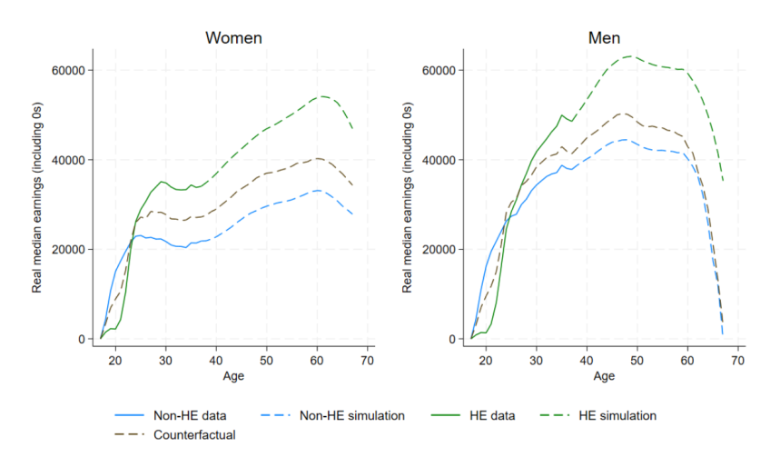
We start by looking at simple plots of median earnings by age. Figure 4.1 shows median pre-tax earnings among graduates and non-graduates, separately by gender. Up to age 37, the earnings are the actual observed earnings for the 2002 GCSE cohort. Beyond age 37, we use the simulated earnings profiles for this cohort, shown as dashed lines.

Figure 4.1. Median actual and simulated gross earnings by age (2002 GCSE cohort)

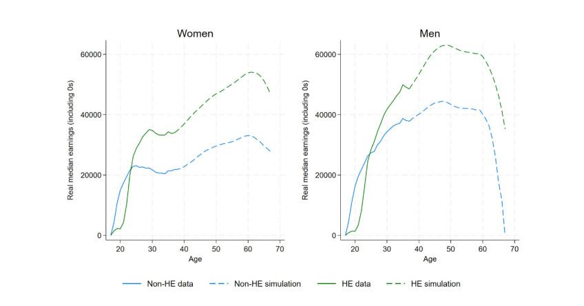
_{Note: Gross annual earnings in 2025/26 CPI prices. Includes zero earnings. Sample selected as discussed in Section 2.1, including minimum GCSE attainment and a Key Stage 5 record. Data before age 27 exclude self-employment earnings. Earnings are uprated to reflect economy-wide real earnings growth between 2004/05 and 2023/24, and by 1.8% per year for every age after 37.}

For both women and men, the median earnings of those who attend HE start below the earnings of those without HE, reflecting that people typically forgo earnings while they study, working fewer hours during their early 20s. The earnings of our HE group saw much stronger growth than those of their non-HE counterparts in their late 20s. This is particularly true for women, as median real earnings amongst female non-graduates in this cohort actually declined slightly after the age of 29. At age 30, median earnings of women HE graduates were around £35,000 (in today’s prices), around 60% higher than the median amongst non-graduate women (£22,000). Median earnings amongst male graduates at age 30 (£42,000 in today’s prices) were over 20% higher than those amongst male non-graduates (£34,000). These patterns match those in Britton et al. (2020), as would be expected given that this report uses the same data up to age 30.

With additional years of tax data, we are now able to describe how the earnings of the same set of graduates actually evolved over the subsequent seven years. Median earnings of male graduates continued to grow strongly between the ages of 30 and 35, by around 20% in real terms, and this growth outstripped the growth for non-HE men (13%). This was in stark contrast to women, who saw very little growth in median real earnings over the same period: median earnings amongst both graduate and non-graduate women were around 1% lower in real terms at age 35 than at age 30. These estimates include individuals with zero earnings in a given year so that year-on-year changes combine changes in real-terms hourly pay, in the number of hours worked and in employment rates. The real-terms decline in annual earnings for women between ages 30 and 35 is more likely to reflect reductions in hours worked over this period, rather than a reduction in hourly pay, although we cannot directly test this using tax data as we do not observe hours worked.

Also of note from Figure 4.1 is the year-on-year decline in real earnings at age 36 which was seen across all groups. This corresponds to the 2022/23 tax year and the ‘cost-of-living’ crisis, a period in which nominal earnings growth across the economy did not keep pace with high CPI inflation.18 There was some bounce-back for female earnings at age 37 (in the 2023/24 tax year) but a further slight real-terms decline in median male earnings in the same year.

Earnings gaps between graduate and non-graduate women were similar at age 37 to what they had been at age 30, and we expect this gap to remain fairly stable at between 50% and 60% for most of their later careers. For men, we expect slightly faster real growth in HE than non-HE earnings up to their late 40s, and then slightly slower declines through the next decade. This means that our predicted HE/non-HE raw earnings gap for men increases steadily from 28% at age 37 to around 45% by age 50, after which it stabilises.

Towards the end of working life, median earnings decline for all groups as people start to reduce their working hours, and more individuals drop out of the labour market altogether as they approach retirement.

4.1 Earnings by subject

Figure 4.2 shows the trajectory of median earnings up to age 37 for the HE group, split by subject, for women and for men. In general, median earnings of female and male graduates in each subject were very similar at age 25, although across all subjects male graduates saw faster real-terms growth in median earnings after that age. After age 25, medicine and economics were the highest-earning subjects, while creative and performing arts were the lowest-earning.

Figure 4.2. Median actual gross earnings by age (2002 GCSE cohort) including zeros: selected subjects

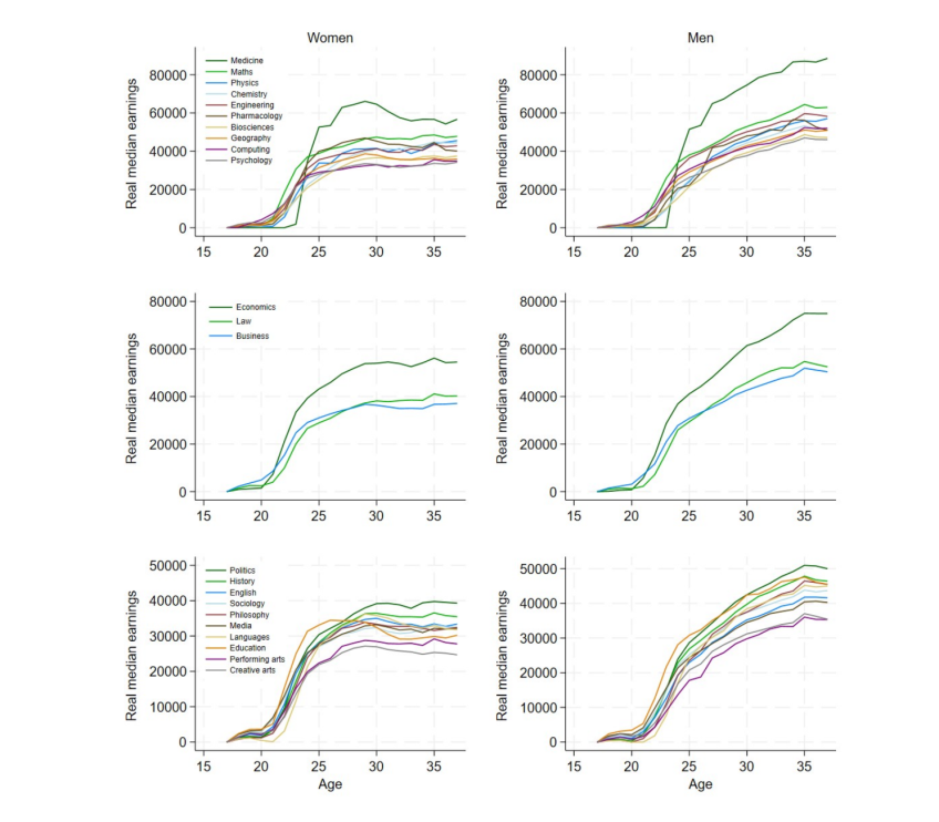
_{Note: Subjects are grouped into STEM subjects (science, technology, engineering and maths), LEM subjects (law, economics and management) and other subjects. Includes zero earnings. Sample selected as discussed in Section 2.1. Data before age 27 excludes self-employment earnings (although we expect this to make little difference to the plot as self-employment earnings for later cohorts are low before age 27).}

Those who studied medicine had near-zero median earnings up to age 23 (reflecting longer courses), but by age 25 they had the highest median earnings of graduates of any subject amongst both men and women. Medicine remained the subject with the highest median earnings for both male and female graduates, although it was almost overtaken by economics for women at ages 35 and 36. This was in part due to a decline in real median earnings of female medicine graduates after age 29, likely due to declines in working hours (male medics continued to see strong growth in median earnings through their 30s).

At age 37, there were large differences in median gross annual earnings between graduates of different subjects. However, there was also substantial variation in earnings amongst graduates of the same subject, which we show in Appendix C. Most notably, the distribution of gross earnings for economics graduates is extremely wide: conditional on having positive earnings, 10% of female economists earn at least £164,000 by age 37 (compared with a median of £68,000), while 10% of male economists with positive earnings earn at least £263,000 (compared with a male economist median of £90,000). This variation is not restricted to the higher-earnings subjects, however; 10% of female creative arts graduates earned at least £61,000, while 10% of male creative artists earned at least £86,000.19 

5. Earnings returns

We now consider the returns to higher education. To do this, we estimate the difference between the gross earnings of those who attended HE and the counterfactual earnings those same individuals may have had if they had not started an undergraduate degree by age 21. As the latter cannot be observed, we predict these based on the regression model discussed in Section 3.2, drawing upon the rich background and prior attainment information from school records. As shown in Figure 5.1, we estimate that our HE group would have had higher counterfactual earnings than our non-HE group, even if they had not in fact attended university: the difference between the non-HE and counterfactual lines reflects the earnings difference attributable to selection into attending university, and the difference between the counterfactual and HE lines represents our estimated gross earnings return at each age.

Figure 5.1. Median actual, simulated and counterfactual gross earnings for our HE and non-HE groups (2002 GCSE cohort) by age

_{Note: ‘HE’ includes those who started a full-time undergraduate degree before the age of 21. Gross annual earnings in 2025/26 CPI prices. Counterfactual earnings estimated as described in Section 3.2. Includes zero earnings. Sample selected as discussed in Section 2.1, including minimum GCSE attainment and a Key Stage 5 record. Data before age 27 exclude self-employment earnings. Earnings are uprated to reflect economy-wide real earnings growth between 2004/05 and 2023/24, and by 1.8% per year for every age after 37.}

These estimates of gross earnings returns reflect earnings simulations for the 2002 GCSE cohort. We then apply today’s tuition fee, student loan and tax policies to these returns, to approximate how the financial return to higher education – and the cost of a degree – would be split between individuals and the exchequer under current government policy. We first look at average returns to attending HE – from the perspective of individuals and the exchequer – before disaggregating these by subject and institution group. We also disaggregate returns by socio-economic status and ethnic group in Appendix J.

5.1 Average net lifetime returns

From the point of view of the student, we estimate that the overall average discounted present value of enrolling in an undergraduate degree is around £90,000 for women and £109,000 for men. In percentage terms, this represents a gain in average net lifetime earnings of around 16% for women and 15% for men.20 As discussed in Section 7, these returns are around a third lower in real terms than those estimated in earlier work.

Figure 5.2 shows how we arrive at these estimates of net individual lifetime returns and Table 5.1 summarises the key numbers. The net individual financial return to HE is the sum of the increase (or decrease) in earnings associated with attending university at each age, minus the increase (or decrease) in taxes paid at each age, plus the value of maintenance loans received and minus the value of any student loan repayments made.21 

Figure 5.2. Decomposition of lifetime individual returns to higher education

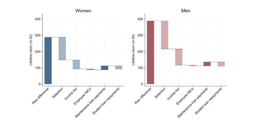
_{Note: All figures are shown in 2025/26 CPI prices, are discounted using Green Book discounting and are mean averages across our HE sample. The first bar shows the raw difference in gross earnings between those who did and did not attend HE. The second bar shows how much of this difference in earnings can be explained by differences in prior attainment and background characteristics. We then account for differences in income tax and employee National Insurance contributions (NICs) as a result of remaining differences in pre-tax earnings. The penultimate bar adds the maintenance loan payments received by students while studying and the last bar takes into account estimated lifetime student loan repayments. Darker bars indicate additions and lighter bars reductions.}

Table 5.1. Average net lifetime earnings differences between graduates and non-graduates and net individual returns

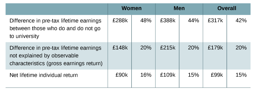
_{Note: All figures are mean averages, shown in 2025/26 CPI prices and discounted using Green Book discounting. Percentages reflect proportional increase relative to non-HE estimates in each case.}

For women, the predicted difference in discounted pre-tax lifetime earnings between those who go to university and those who do not is around £288,000. We estimate that approximately half of that difference can be explained by the different observable characteristics of women who attended HE (we refer to this as ‘selection’ in the figure). That is, we estimate that women who go to university earn around £148,000 more pre-tax than if they had not gone to university; this is the gross lifetime earnings return. Accounting for additional income tax and payments of employee National Insurance on these higher earnings reduces the net individual returns by roughly another £60,000. Including the student loan system slightly increases the return by around £2,000, as we estimate women repay slightly less, on average, in overall student loan repayments (£22,000) than they receive in maintenance loans (£24,000). This results in a final estimated net lifetime return of £90,000 for women.

For men, the predicted difference in raw pre-tax earnings for those who do and do not attend university is greater than for women, at around £388,000. However, the difference that can be explained by observable characteristics is also somewhat bigger, taking the gross return to around £215,000 on average for men. Since much of the additional income later in life will be subject to the higher rate of income tax, the difference in income tax reduces the net return by £99,000 for men; the difference in employee National Insurance payments is much smaller (£4,000). We estimate that men will make student loan repayments of around £27,000 on average, exceeding in present-value terms the average maintenance loans they receive (£24,000), leaving a total average net lifetime return of £109,000 for men.22 

We now turn to estimating the equivalent average returns to the exchequer, i.e. from the point of view of the taxpayer. These consist of the increase in lifetime tax and National Insurance receipts (including both employee and employer NICs), minus any up-front spending on teaching grants and initial outlay on tuition fee and maintenance loans that is not offset by future student loan repayments.23 We estimate there are average lifetime exchequer returns of £48,000 for women and £107,000 for men – which should be interpreted as the average gain to the exchequer from people enrolling in the courses that they did in fact enrol in, compared with not going to university at all.

Figure 5.3 shows the different components of exchequer outlays and returns for women and men. Financing an undergraduate degree costs the exchequer around £55,000 for both women and men in tuition and maintenance loan payments and teaching grants.24 Women will only pay back around 40% of that total up-front cost in student loan repayments, but the higher income tax payments of graduate women more than offset the remaining cost to the exchequer represented by the 60% of initial outlay which is not recovered through loan repayments.25 Adding the additional employee and employer NICs – around £5,000 and £22,000 respectively – leads to the overall figure for the average net exchequer return to HE for women of £48,000 per student.

Figure 5.3. Decomposition of lifetime exchequer returns to higher education

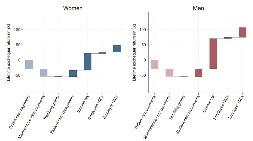
_{Note: All figures are shown in 2025/26 CPI prices, are discounted using Green Book discounting and are mean averages across our HE sample. The first two bars show the net present value of tuition fee and maintenance loan outlay. The next bar shows the net present value of teaching grants for high-cost subjects. Subsequent bars then show the net present value of government receipts in terms of student loan repayments and higher income tax and National Insurance payments as a result of differences in pre-tax earnings that cannot be explained by differences in prior attainment and background characteristics. Darker bars indicate additions and lighter bars reductions.}

Financing a degree costs essentially the same for men as for women but, due to their higher average earnings, men are expected to pay back a larger fraction (around 48%) of that cost in present-value terms through student loan repayments. The increase in income tax payments is the most important part of the exchequer return for men; along with additional receipts of employee and particularly employer NICs, tax receipts increase by around £136,000 per student, resulting in an overall average net exchequer return to HE for men of £107,000 per student.

Figure 5.4 shows cumulative average returns by age – both for individuals and for the exchequer. The figures at age 67, with Green Book discounting applied (the darker lines), correspond to the average lifetime estimates discussed in the text above.

Figure 5.4. Mean cumulative individual and exchequer returns to higher education by age

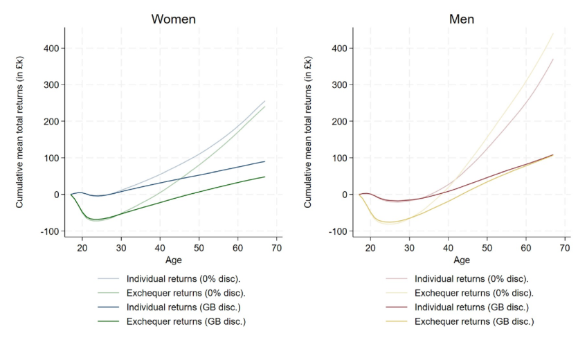
_{Note: All figures are shown in 2025/26 CPI prices and are discounted using either Green Book (GB) discounting, as in our main estimates, or with a 0% real discount rate. Returns at a given age are discounted cumulative returns to that age.}

Several aspects of the graphs are notable. First, while the cumulative discounted returns to women from attending university are positive on average from age 27, for men this is only true from age 38. This mainly reflects that men experience lower earnings returns in their 20s than women (who have worse counterfactual, non-HE earnings). Both individual and exchequer returns for men grow more strongly than for women later in life and exceed returns for women by age 55.

Second, the size of the estimated cumulative returns figures is dramatically affected by the choice of discount rate. With 0% real discounting, net individual lifetime returns would be £256,000 for women and £371,000 for men (compared with £90,000 and £109,000 with Green Book discounting).26 Men’s projected lifetime returns in cash terms exceed those of women, but the difference is much larger with a lower discount rate.

Third, HE is a long-run investment from the point of view of the taxpayer. Exchequer returns are substantially negative early in people’s careers – reaching around minus £70,000 (with Green Book discounting) on average by their early 20s for both genders – and remain negative on average for a significant part of the life cycle. This is because the exchequer bears almost all of the up-front cost of financing HE in the form of student loan outlay (whereas maintenance loan payments partly compensate students for forgone earnings while studying). With Green Book discounting, exchequer returns only turn positive at age 44 for men and age 48 for women. With 0% discounting – which places more relative value on earnings increases later in the life cycle – the equivalent ages are 39 and 40.

These averages hide substantial heterogeneity amongst graduates, as shown in Figure 5.5, which presents our estimates of the distribution of lifetime individual and exchequer returns, for women and for men. We expect the 10% of women with the highest returns to each gain more than £230,000 net of taxes and loans, but that around 19% of women will not get a positive net lifetime return from their degree at all. For men the differences are even larger: we expect the 10% of men with the highest returns will each gain more than £330,000, but around 31% of men can expect a negative net individual lifetime return. We therefore estimate that 24% of graduates will not gain financially from attending HE (up slightly from the estimate of one-in-five in Britton et al. (2020), for reasons discussed in Chapter 7). We estimate that the 10% of women with the lowest net lifetime returns are more than £30,000 worse off, while 10% of men can expect to be more than £90,000 worse off over their lifetimes.

Figure 5.5. Distribution of net individual and exchequer returns to higher education

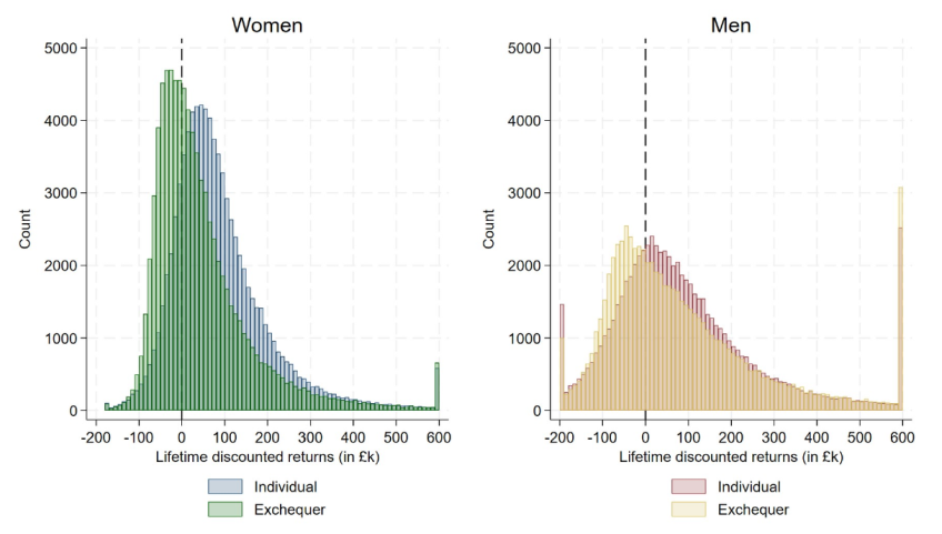
_{Note: All figures are shown in 2025/26 CPI prices and are discounted using Green Book discounting. Results have been censored to comply with statistical disclosure rules around reporting results for small sample sizes. Lower counts for men reflect that the spread of returns is much wider amongst men; total counts for women and men are consistent with sample sizes for our HE group in Table A.1 in Appendix A.}

For both men and women, exchequer returns are lower than individual returns. We expect the 10% of women with the highest exchequer returns to each generate more than £190,000 for the exchequer as a result of going to university, but around 42% of all women to generate negative exchequer returns. For men, we estimate that the 10% with the highest returns will each contribute more than £360,000 to the exchequer as a result of attending HE, but the exchequer will make an overall loss on the undergraduate degrees of around 39% of men.

Table 5.2 summarises the mean and median lifetime returns to HE, and the share of individuals achieving positive returns. The median returns are positive for women and for men, both to the individual and to the exchequer, albeit notably lower than the mean. This reflects graduates at the top of the earnings distribution – especially men – accumulating particularly high returns and pushing up the mean.27 For estimates of total returns to HE across both the individual and the exchequer, see Appendix D.

Table 5.2. Average individual and exchequer lifetime returns, and share achieving positive returns, for women and for men

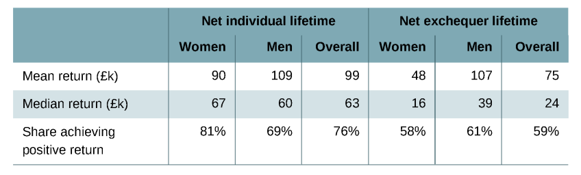
_{Note: All figures are shown in 2025/26 CPI prices and are discounted using Green Book discounting.}

5.2 Lifetime returns by subject and institution type

Figure 5.6 presents results on the distribution of net individual lifetime returns by subject studied for women. Estimated discounted average returns range from close to zero for creative and performing arts and languages to close to £200,000 for business, medical sciences and law, over £300,000 for economics and over £400,000 for medicine.28 The estimated range of individual returns is larger for subjects that have higher average returns. Notably, there are many subjects that have relatively low average returns for women, but from which almost all women who studied them are projected to achieve positive returns.29 

Figure 5.6. Net individual lifetime returns to higher education for women, by subject

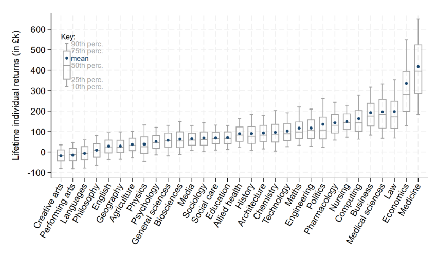
_{Note: All figures are shown in 2025/26 CPI prices and are discounted using Green Book discounting. Subject classification reflects CAH2 and excludes a small number of subjects due to low sample sizes. Subjects are ordered by mean average returns.}

Figure 5.7 presents net individual lifetime returns by subject studied for men. Returns vary more by subject for men, with strongly negative estimated returns for performing and creative arts and social care, on average, and negative estimated returns for the vast majority of men who studied these subjects. Average net individual returns are close to zero for men across a wide range of (predominantly humanities) subjects. The subjects with the highest average lifetime returns for men are medicine (close to £500,000) and economics (over £650,000) – with particularly high expected returns for a small number of men who studied economics driving up the mean return (compared with the median of around £450,000).

Figure 5.7. Net individual lifetime returns to higher education for men, by subject

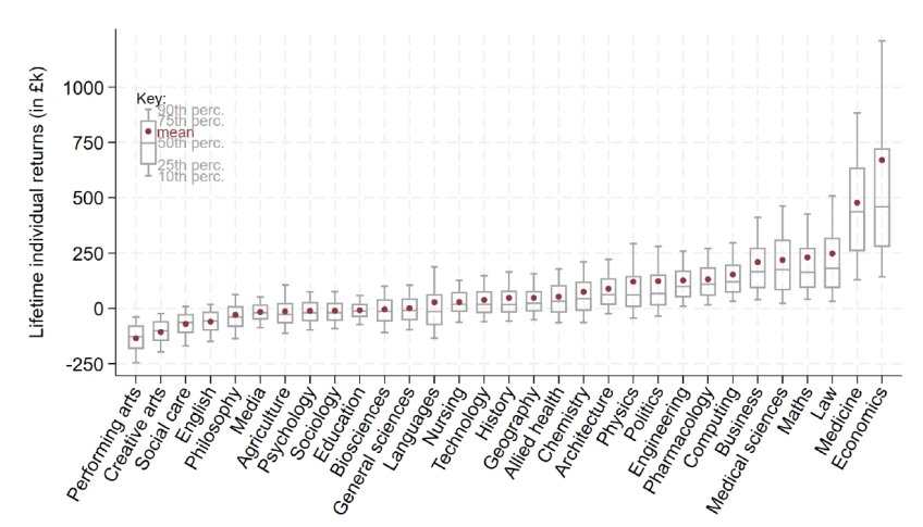
_{Note: See note to Figure 5.6. The ranges of the vertical axes differ between the two charts.}

Subjects that are associated with higher earnings do not necessarily have higher returns, because the counterfactual earnings of students also differ by subject studied: the students of some subjects have more favourable background conditions than others (such as higher prior attainment) which affect how much they could have earned had they chosen not to go to university. This partly explains, for instance, why women who study physics can be both relatively high-earning over their careers and have relatively low average individual returns, as shown in Figure 5.8.30 The opposite is true for social care, which offers solid returns for most women despite the comparatively low earnings of graduates.

Figure 5.8. Net individual lifetime returns versus discounted lifetime gross earnings, by subject and institution type

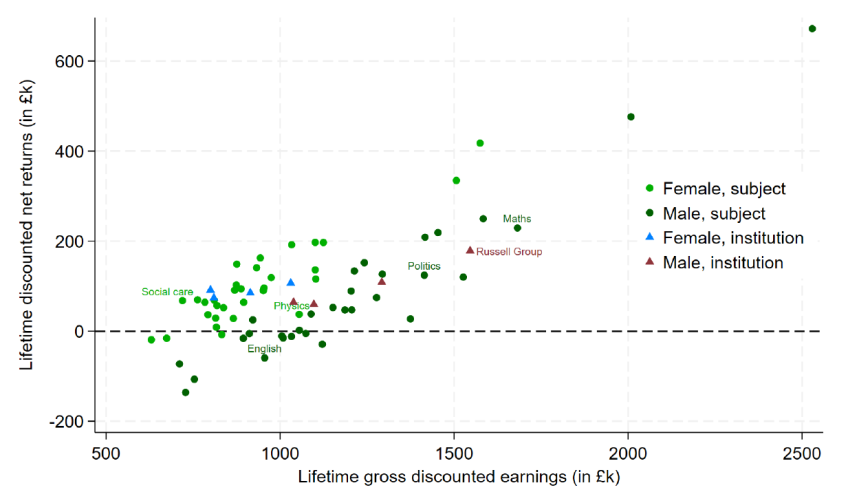
_{Note: See note to Figure 5.2 for details on calculation of lifetime discounted returns to the individual, shown on the vertical axis. The horizontal axis shows mean average lifetime earnings prior to taxes and student loan repayments, also discounted using Green Book discounting.}

Figure 5.9 shows the distribution of net individual lifetime returns amongst students who attended different types of institution. While there are differences in gross earnings between women attending different university types, there is little difference between average lifetime returns across university types for women. The returns for women attending pre-1992 and other universities are fairly similar, with average returns for women at Russell Group universities around a quarter higher (£107,000). Within all types, more than three-quarters of women benefit from attending HE. The pattern for men is somewhat different, with differences in average returns between men at Russell Group universities (£178,000), pre-1992 universities (£109,000) and other universities (£60,000 and £64,000 amongst more and less selective).31 We estimate a sizeable minority of men who attended pre-1992 or other universities will experience negative returns in discounted net present-value terms from attending HE.

Figure 5.9. Net individual lifetime returns to higher education by institution type

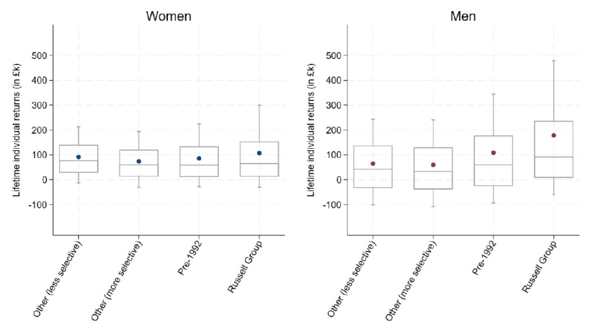
_{Note: Institutions are divided into four groups: Russell Group; old (pre-1992) universities not in the Russell Group; and an ‘other’ category which splits the remaining universities into more and less selective based on the average GCSE point scores of those attending these universities for full-time undergraduate degrees beginning between ages 18 and 20 from the 2002–07 GCSE cohorts.}

As shown in Figure 5.10, average exchequer returns by subject are generally well correlated with individual returns: subjects that are higher-return from the perspective of students also tend to be higher-return for the exchequer. A number of subjects for men have both negative individual and exchequer returns for men on average (as shown in the lower-left quadrant of the chart). These include performing arts, creative arts, social care, English, philosophy, sociology, media, psychology, education, agriculture and biosciences. For women, there are fewer subject areas with negative individual returns, but there are a handful in the upper-left quadrant that have positive individual returns on average but negative returns for the exchequer. Average individual and exchequer returns by institution type are also well correlated (shown by triangles on the chart). All averages by institution type are in the upper-right quadrant: both students and the exchequer gain on average from attending all four types of institution, among both men and women. Figures showing the distribution of exchequer returns by subject and by institution type are included in Appendix F.

Figure 5.10. Net individual versus exchequer lifetime returns, by subject and institution type

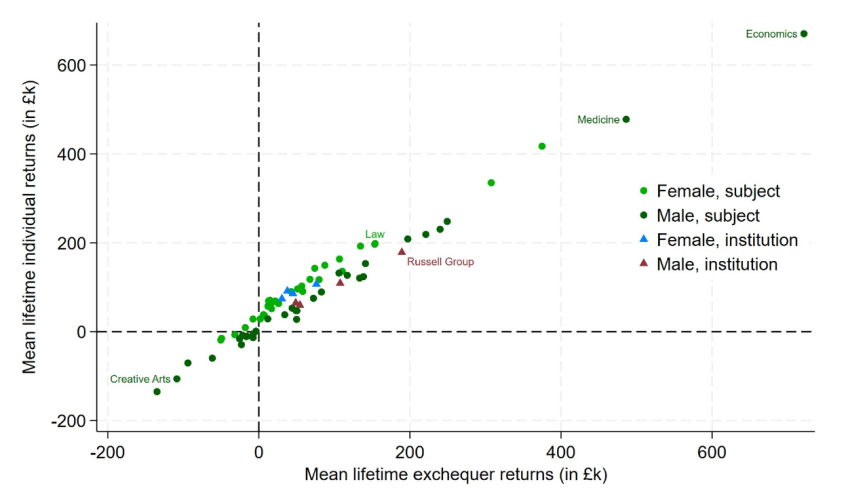
_{Note: See notes to Figures 5.2 and 5.3 for details on calculation of lifetime discounted returns to the individual and the exchequer. Each circle represents an average by subject and gender (e.g. women studying law) and each triangle represents an average by institution group and gender (e.g. men at Russell Group universities).}

6. How robust are these estimates, and what are the limitations?

We estimate the returns to undergraduate degrees for England-domiciled students over the course of their working lives, drawing primarily on information about the earnings of individuals who took their GCSEs in 2002 and who entered the higher education sector in the mid to late 2000s. We simulate earnings profiles for the remainder of their working lives and then estimate individual and exchequer returns under current government policy on taxes and student loans, including assumptions about future government policy. This is not a straightforward exercise and the resulting estimates are subject to important limitations and several sources of uncertainty. The caveats discussed here should be carefully considered, particularly when using the estimates to inform prospective students deciding whether to attend HE today. In this chapter, we first discuss the conceptual limitations of our approach and then assess how sensitive our main estimates are to alternative modelling decisions.

6.1 Limitations of our estimates

Estimating causal effects

As was the case in Britton et al. (2020), our approach relies on controlling for observable characteristics that are correlated both with earnings and with selection into attending HE. We draw on rich background information from the National Pupil Database, including information on students’ socio-economic background, demographic characteristics and prior attainment (including at Key Stages 2, 4 and 5) to control for the influence of a large array of potential confounding factors. This is a substantial improvement on comparisons of average earnings of graduates and non-graduates, and these observable controls do capture a large amount of selection – as illustrated in Figure 5.1.

However, our methodology is unlikely to recover the precise causal effect of attending HE for the cohorts we study. In particular, there may be other unobserved characteristics that both determine selection into HE and degree choice, and have an independent effect on earnings. In theory, this bias could go in either direction. On the one hand, unobserved characteristics such as ambition might make people more likely to go to university and might have an independent positive effect on earnings. This would lead to higher estimated returns to HE using our method than the true causal return. On the other hand, the people who attend university may be those who have weak earnings prospects without a degree and expect to gain a lot from attending. This is known as selection on gains, and would imply – all else equal – that the earnings of the non-HE group are systematically higher than the counterfactual non-HE earnings of our HE group. If this selection is based on characteristics we do not observe, this may lead us to overestimate the counterfactual earnings of our HE group and lead to a lower estimated return than the true causal effect.

Furthermore, the direction and magnitude of this bias may also vary across subjects and institution types. A notable example is students who choose subjects such as creative and performing arts. These students are likely to differ in unobserved ways from those who choose not to go to university, beyond the characteristics we can measure. For example, they may systematically place less weight on labour market earnings than those with similar observed characteristics who did not go to university, which would mean our estimates understate the true returns to these subjects. More generally, where selection into a particular subject or institution type is correlated with preferences or characteristics that also affect earnings, the bias in our estimates may be larger than for the average graduate.

Estimation based on a cohort that attended higher education two decades ago

The gross earnings returns we estimate are for a specific cohort born in the mid 1980s who went to university in the mid 2000s. We have then adjusted their earnings and applied the parameters of the tax and student loans systems so that the split of gross earnings returns and the cost of a degree between individuals and the exchequer reflects the policies facing people enrolling at university in 2025. However, for these estimates to be a good guide to net lifetime returns for students attending university today, three sets of assumptions must hold: that gross returns to specific degrees and institutions have not changed since the 2002 GCSE cohort; that the future earnings trajectories of the 2002 cohort, which we simulate, are a reasonable approximation of what later cohorts will experience; and that the tax and student loan policies we apply would not themselves have altered the choices and earnings of the 2002 cohort. Each assumption is open to challenge.

Changes to the HE landscape. The HE sector has expanded substantially in recent decades, although the implications of this for returns are ambiguous. All else equal, the increase in supply of graduates would be expected to lead to lower returns to HE for later cohorts. But other factors complicate that picture. The expansion has been concentrated amongst students with lower GCSE attainment, who may experience different returns from those of their higher-attaining counterparts (we look at this group specifically in Chapter 8); the role of an undergraduate degree in signalling an individual’s underlying ability to potential employers may also have shifted. The expansion has also not been equally spread across subjects and institutions, affecting both overall returns and the relative returns to different course choices. Demand-side changes are similarly ambiguous: shifts in the composition of the UK economy or changes in technology might have made certain skills more valuable and others redundant, and these shifts may themselves be influenced by changes in the supply of graduates. In Chapter 9, we document changes in the supply of graduates over time, and illustrate how returns to degrees may already have changed for more recent cohorts. We do not attempt to model how returns may change for future cohorts.

Simulating later-life earnings. Any returns estimates that are forward-looking will be subject to uncertainty about the future. We do not know whether the earnings trajectories of future graduates will be similar to those of past graduates, what will happen to economy-wide earnings growth, and what retirement patterns are going to look like in 50 years’ time. Where they are available, we use official economic forecasts produced by the Office for Budget Responsibility, most importantly for long-run economy-wide real average earnings growth. But like all long-term economic forecasts, these are subject to substantial uncertainty. This partly explains why our estimates differ from those of Britton et al. (2020); since that report was published, earnings and employment have evolved differently from what was previously expected, with a global pandemic and a ‘cost-of-living’ crisis which were not foreseen in February 2020. Life-cycle earnings dynamics may also differ for later cohorts: patterns of worklessness amongst women have shifted as the age of first childbirth has risen, for example.32 These issues are more acute for later ages, where the gap between the cohorts whose returns we are trying to predict and those whose data we use in estimation is particularly large. Discounting mitigates this problem to some extent as earnings and returns at later ages receive a lower weighting in our lifetime estimates. We do not attempt to model the potential impact of major social and economic trends, such as changes in healthy life expectancy or the adoption of AI.

Policy modelling. To make our estimates more relevant for policymakers today, we apply today’s tax and student loan policies, estimating individual and exchequer returns as if the cohort we study had been aged 18 in 2025/26 instead of 2003/04. We reflect current stated government policy as to how these systems will evolve in the coming years but, as shown in Chapter 7, changes to government policy can have a substantial impact on how gross earnings returns translate into individual and exchequer returns. Our approach also implicitly assumes that a different policy environment would not have changed the choice to attend HE or the subsequent earnings of those who did. In practice, differences in marginal effective tax rates might affect labour supply decisions, for instance.33 Changes in up-front spending on teaching or in the design of student support might affect which students enrol or their outcomes. We do not speak directly to these possible effects, though in Chapter 9 we compare returns for successive cohorts of graduates, some of whom entered HE following the most substantive changes to tuition fees and the student loan system.

Focus on earnings

Estimates of the individual and exchequer returns to HE as a result of impacts on lifetime earnings and employment do not provide a complete picture as to the impacts of HE that individuals – or policymakers – might be interested in. Some of the impact of attending HE on earnings likely results from human capital accumulation that makes workers more productive and is rewarded in the labour market. But if attaining a degree yields private returns by signalling something to employers (about an individual’s underlying ability or other attributes) without making individuals more productive, the private return may exceed the social return, since signalling does not generate productivity gains for the wider economy. We do not take any stance on the relative importance of these channels in the earnings impacts we find.

Further, our results show only the earnings benefit of HE for individuals and (some of) the tax benefits for government of those higher earnings (and higher loan repayments), net of the cost of financing HE. We measure annual taxable earnings over working life and so will not capture differences in hours worked or in pension saving (particularly employer pension contributions), both of which are likely to be higher amongst graduates. Importantly, we do not consider potential non-financial impacts such as on marriage, fertility, social networks, health, happiness or job satisfaction, which may constitute an important part of the private return to HE, nor any potential spillovers to others of having a more educated population. We also do not account for some potential fiscal consequences (such as additional revenues from lower spending on unemployment benefits or changes in demand for particular public services). All of these factors mean that our estimates are not sufficient to determine the socially optimal level of participation or investment (public or private) in HE.

What these estimates can and cannot tell us about policy

We estimate returns to university courses and institutions for students who actually enrolled in those courses. Our results should not be interpreted as the returns that would be realised if the HE sector were significantly expanded or contracted, or if students were reallocated across courses and universities. We do not estimate counterfactual earnings for non-graduates had they attended HE and cannot infer what the returns might be for students who did not enrol, whose characteristics would likely differ from those of the average graduate. We also do not model broader knock-on effects on the labour market from individuals’ choice of course or university.

In practice, if some graduates had instead chosen not to attend HE or had chosen a different course, students may have redistributed in complex ways across subjects and universities, and the labour market may have adjusted, potentially changing the returns. These are referred to as general equilibrium effects and they are not captured by our approach. Our estimates are therefore informative about the average lifetime returns experienced by those who attend HE, but they are not a guide to the consequences of major changes to the sector. Policy decisions on those questions require additional analysis that we do not undertake here.

6.2 Sensitivity to alternative assumptions

In this section, we discuss how different modelling decisions might change our estimates. We focus on how sensitive our estimated average net individual lifetime returns are, summarising these results in Table 6.1. The effects of the same sensitivity tests on average exchequer returns are presented in Appendix G.

Table 6.1. Average net individual lifetime returns, and share achieving positive net individual lifetime returns, by sex, under different modelling assumptions

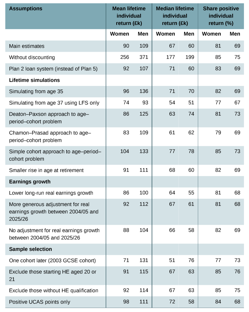
_{Note: Each alternative assumption is applied separately, not in combination. The approach to estimating earnings profiles by age from Deaton and Paxson (1994) takes a cohort view, but allows for period effects that are orthogonal to a time trend. The Chamon and Prasad (2010) approach takes a period view and allows for cohort effects that are orthogonal to a time trend.}

Discounting and loan policy

As shown in Figure 5.4, our estimates are very sensitive to the choice of discount rate: the relative value of a unit of income received today compared with further in the future. Our main estimates apply the Green Book’s recommended discount rate of 3.5% (and then 3.0%) to express lifetime returns in terms of earnings at age 18. If we instead apply a 0% real discount rate – adjusting earnings in future years for inflation but applying no further adjustment to reflect time preferences – then our estimated net lifetime returns are substantially higher at £256,000 for women and £371,000 for men on average (instead of £90,000 and £109,000 respectively).

In contrast, our estimates of lifetime returns are not very sensitive to the decision to model student loan repayments under the ‘Plan 5’ student loan terms available to undergraduate students starting courses in 2025/26. If we instead model ‘Plan 2’ student loan terms (as were available to England-domiciled undergraduates who started courses between 2012/13 and 2022/23), our estimates of lifetime returns increase slightly for women and decrease slightly for men. This is consistent with lower average earnings amongst women: the higher repayment threshold, shorter repayment period and higher interest rate associated with Plan 2 loans mean lower earners can expect to repay less under Plan 2 loan terms, and higher earners to repay more. However, while estimated average lifetime returns do not differ substantially between the loans, differences in lifetime repayments for specific individuals may be substantial.

Lifetime simulations

Since they use the distribution of earnings at age 37 as a starting point, our lifetime earnings simulations may be particularly sensitive to earnings in the most recent tax year (2023/24). As illustrated in Figure 4.1, median real earnings declined between ages 35 and 36 due to high CPI inflation in 2022/23. If we instead simulate earnings from age 35, ignoring earnings observations in 2022/23 and 2023/24, this increases our estimated average net lifetime returns by around £6,000 for women and £27,000 for men. This is consistent with graduate men seeing the largest decrease to real earnings in the most recent years of the Longitudinal Education Outcomes data. However, the share with positive lifetime returns changes little.

Our main estimates use HESA–HMRC data to simulate earnings for graduates between the ages of 38 and 44. We prefer to use these administrative data, which are likely to be more reliable than survey data, but this means using information on more recent birth cohorts to model graduates’ earnings in their early 40s than we do for non-graduates’ earnings. If we instead use the Labour Force Survey for both graduates and non-graduates from age 37, our estimates of average lifetime returns decrease by around £16,000 for both men and women.

We also model three alternatives to constructing age–earnings profiles from the HESA–HMRC and LFS data. Our main estimates take a ‘simple period view’: we effectively assume that there are no cohort effects, and attribute earnings differences across cohorts in a given year to age effects rather than to cohort effects. One alternative would be to assume there are no period effects, instead ascribing variation in earnings between adjacent periods for those in the same cohort to age effects. We call this the ‘simple cohort view’. Taking the simple cohort view leads to higher average lifetime returns for both women (£104,000) and men (£133,000). More complex alternatives to each of the period and cohort views would instead impose not that the other effect was zero, but that it was orthogonal to a time trend; the first papers in the literature using these techniques were Deaton and Paxson (1994) for the cohort view and Chamon and Prasad (2010) for the period view. The Deaton–Paxson and Chamon–Prasad approaches produce slightly lower estimates of lifetime returns for women, and higher estimates for men.34 See Appendix G for further discussion of these different approaches.

Another concern is that our assumptions around changes in retirement patterns across cohorts may now overestimate retirement ages for the 2002 GCSE cohort, especially given slower growth in life expectancy and declines in healthy life expectancy since the pre-pandemic period (Department for Work and Pensions, 2025). In our main estimates, we fix model parameters for eight years at age 51, with parameters from ages 60 to 67 corresponding to ages 52 to 59 in the data. This is the same approach as was taken by Britton et al. (2020). Instead freezing parameters for eight years at age 59 – allowing employment rates to decline during their 50s in the same way as they did among much older cohorts – does not notably change our results on lifetime returns.35 

Earnings growth

Our simulations also require assumptions about long-run real earnings growth, which we use to uprate our simulated future earnings – reintroducing forecast period effects. For our main estimates, we assume CPI-real earnings growth of 1.83% per year after age 37, in line with the OBR’s most recent published figures as of April 2026. The OBR has since published updated long-run projections, although the downgrade (to 1.75% per year) is small enough that we do not expect it to materially affect our estimates (see footnote 10). Indeed, we show the sensitivity of our results to an even less generous earnings growth assumption of 1.2% per year – the same as was used in Britton et al. (2020). This leads to a modest reduction in estimated lifetime returns.

We also rely on historical earnings growth data to account for real earnings growth observed since 2004/05 – the year in which the 2002 GCSE cohort were aged 18. We show that our results are not particularly sensitive either to using a more generous index of earnings growth for this adjustment or to not uprating for growth between these cohorts at all.36 

Sample selection

Our main estimates are based on the 2002 GCSE cohort, the earliest cohort for which we have the fully linked administrative data, and so for which we can observe earnings at the oldest age. However, match rates between the education and tax data are marginally worse for this cohort than for later cohorts. If we instead use one cohort later (the 2003 GCSE cohort) and begin our simulations from age 36, our estimated net individual lifetime returns increase by around £22,000 for men, but decrease by around £19,000 for women. In Section 9.3, we explore further whether returns at a specific age have changed for successive cohorts.

Finally, we must make many decisions about who to include in or exclude from our main estimation sample. For instance, we choose to include students who begin full-time undergraduate degrees by age 21 in our HE sample, and drop later entrants from the sample outright. If we instead focus only on those who begin degrees by age 19, we estimate slightly higher average returns. Our main estimates include all those we observe starting an undergraduate degree in our data – whether or not they actually complete a degree. Excluding those for whom we do not eventually observe a degree qualification in the HESA data also leads to a modest increase in estimated returns. Another important restriction we decide on is to only include individuals who are observed with a Key Stage 5 record in Year 13. This includes a non-trivial number of students who are observed with a record, but for whom we do not observe any actual exam grades. We test the sensitivity of our results to requiring students to have positive UCAS points in the school data. This leads to a small increase in estimated returns, particularly for women.

7. How do these estimates compare with previous estimates?

Both this report and Britton et al. (2020) estimate lifetime returns to undergraduate degrees, focusing on the 2002 GCSE cohort, using the Longitudinal Education Outcomes, HESA–HMRC and Labour Force Survey data, and applying very similar methodologies. In this chapter, we discuss how and why our headline estimates have changed, and then turn to our estimates of returns by subject.

7.1 Overall individual and exchequer returns

Our headline estimates are lower than those in Britton et al. (2020), as shown in Table 7.1. For men, the central estimates of average individual and exchequer returns are down by 35% and 29% respectively relative to those in Britton et al. (2020), after they have been converted to 2025/26 prices. For women, the estimate for individual returns is down by 29%, while exchequer returns are 9% higher.

Table 7.1. Comparison of average net lifetime returns estimates between Britton et al. (2020) and this report

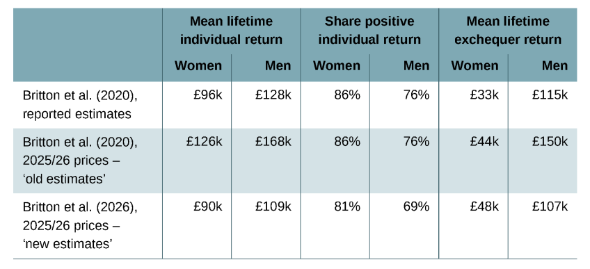
_{Note: All figures are discounted using Green Book discounting. ‘Britton et al. (2020), 2025/26 prices’ adjust for forecast CPI and average economy-wide real earnings growth between 2018/19 and 2025/26. ‘Britton et al. (2026) 2025/26 prices’ match mean average lifetime returns presented in Table 5.2.}

The estimates have changed for two main reasons: first, earnings growth for graduates in the 2002 GCSE cohort between the ages of 30 and 37 has disappointed relative to our previous simulations; and second, changes in government policy around taxes, how higher education is financed and student loans have seen an increasing share of the overall return to HE captured by the exchequer, rather than graduates. We decompose the overall changes in individual and exchequer lifetime returns respectively in Figure 7.1, which tracks the ‘old estimates’ from Britton et al. (2020) through to the new estimates presented in this report. In each figure, the darker shaded bars represent the changes that have increased returns relative to the previous estimates, while the lighter bars represent changes that have reduced the returns.

Figure 7.1. Decomposition of changes in average net individual and exchequer lifetime returns between Britton et al. (2020) and this report, 2025/26 prices

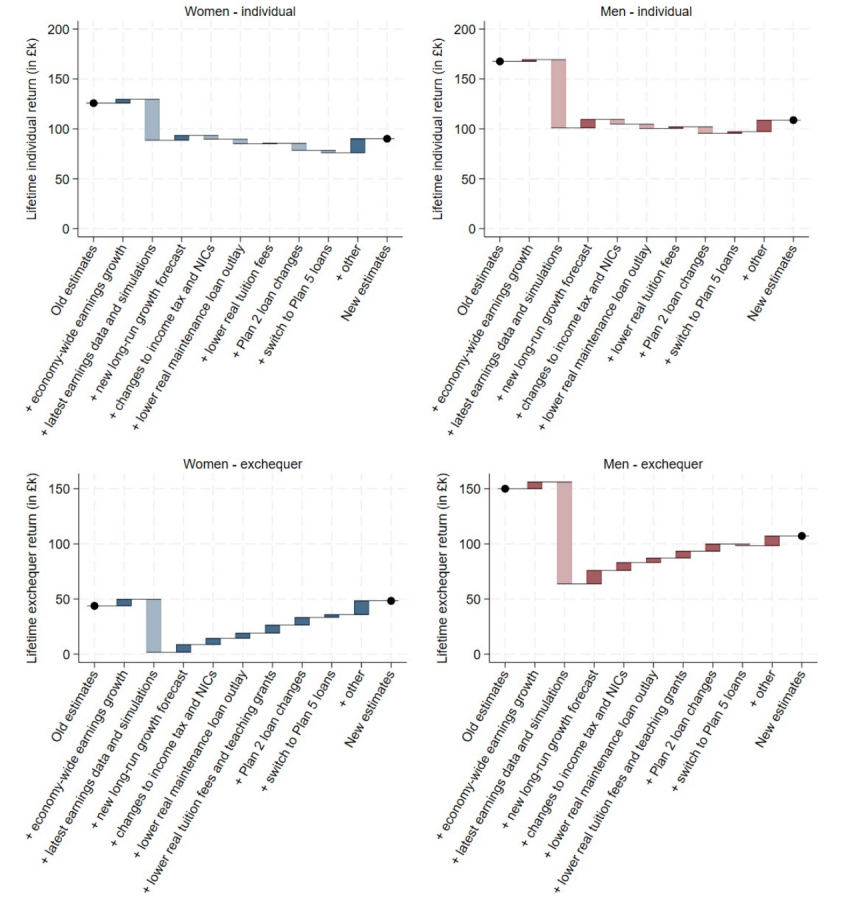
_{Note: All figures are shown in 2025/26 CPI prices, are discounted using Green Book discounting and are mean averages. Darker bars indicate additions and lighter bars reductions, from left to right. In practice, we estimate this decomposition from right to left. We start from our latest headline results, then cumulatively impose assumptions used in our previous estimates, in the following order: (1) switch from the Plan 5 loan system to the current Plan 2 system; (2) switch from the current Plan 2 system to that which would have been in place under government policy as of 2019/20 (with repayment and interest thresholds set to increase with average earnings each year); (3) higher real-terms tuition fees (and tuition fee outlay) and high-cost course funding; (4) higher real-terms maintenance loans; (5) reflect the tax thresholds and rates (income tax and National Insurance contributions) applying in 2019/20 in 2025/26 prices; (6) apply a lower long-run real earnings growth rate (1.2% per year, as used in Britton et al. (2020)); (7) assign individuals their previously simulated earnings for ages 31 to 67; and (8) remove estimated real earnings growth between 2018/19 and 2025/26. In each case, we re-estimate counterfactual earnings and recalculate lifetime returns. The ‘other’ bar is the remaining gap between our estimates from step (8) and the headline results from Britton et al. (2020).}

The first bar represents economy-wide earnings growth that has occurred between 2018/19 and 2025/26. This should not be thought of as a revision to the estimates; rather it is an artefact of the fact that we are simulating from a later point in time than in Britton et al. (2020) and estimating net returns that are intended to be relevant for a later cohort. In any case, this real earnings growth represents a small share of the overall change.

The second, and most important, bar in these plots represents updates to our simulations based on the additional data that have become available since Britton et al. (2020). We now observe seven extra years of earnings in the LEO data (up to 2023/24, where previously we only observed earnings up to tax year 2016/17), meaning we now observe the 2002 GCSE cohort up to age 37 rather than age 30. Actual earnings growth for graduates in this cohort between the ages of 30 and 37 was towards the bottom of the plausible range considered in Britton et al. (2020). This partly reflects unforeseen shocks to real earnings, including as a result of economic disruption around the COVID-19 pandemic and then the ‘cost-of-living’ crisis.37 For non-graduates, this disappointing earnings growth was offset by increases in the minimum wage and by lower levels of worklessness than had previously been forecast for non-graduate women. These differences can be seen in Figure 7.2.

Figure 7.2. Comparison of actual and simulated median gross earnings (excluding zeros) and worklessness rates over the life cycle for graduates and non-graduates

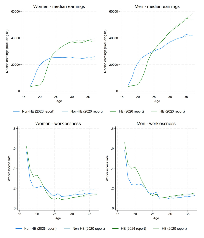
_{Note: Top panel shows median gross annual earnings in 2025/26 CPI prices, excluding zero earnings. Data before age 27 exclude self-employment earnings. Bottom panel shows the share of individuals with zero earnings at a given age. Dotted lines reflect simulated data from Britton et al. (2020). To make our series as comparable as possible, we only include individuals appearing both in our analytical sample and in the sample used by Britton et al. (2020). ‘HE’ in both reports includes only those who started full-time undergraduate degrees before age 21. We also do not uprate earnings to reflect economy-wide real earnings growth between 2004/05 and 2023/24. This figure is therefore not directly comparable to Figure 4.1.}

Since our simulations are calibrated on the final year of earnings in the LEO data, graduates’ earnings trajectories in their 30s and their age-37 earnings in particular also matter meaningfully for projected earnings throughout the rest of the life cycle.38 Overall, incorporating new earnings data into our simulations accounts for a reduction in average net individual lifetime returns of approximately £41,000 (32%) for women and £68,000 (40%) for men. Absent changes to government policy since 2019, this would have approximately wiped out the entire average exchequer return for women (see the bottom left panel of Figure 7.1).

The third bar accounts for changes in how we model long-term real earnings growth over time (in addition to earnings growth associated with increases in age and experience). Reflecting more recent OBR forecasts for long-term real growth in average weekly earnings leads to a small increase in the estimated returns relative to previous estimates.39

The remaining bars represent the impact of policy changes between 2019/20 and 2025/26. These include: the tax revenues associated with a given change in earnings; the up-front cost of financing higher education; and the share of those up-front costs that is expected to be borne by individuals through student loan repayments.

On the tax side, income tax thresholds were around a fifth lower in real terms in 2025/26 than they had been in 2019/20. They are set to remain at the same cash levels until April 2031, which will constitute a further 9% real-terms decrease in the thresholds relative to previous modelling from 2030/31 onwards, increasing the income tax paid at any given level of earnings.40 While this will increase estimated income tax payments from individuals whether or not they went to higher education, it will mean that any given increase in gross earnings associated with attending HE is associated with a lower net individual return and a higher exchequer return as more of any earnings return accrues to the exchequer. Changes to rates and thresholds for employee and employer National Insurance contributions since 2019/20 will have slightly increased our estimate of net individual returns (which only reflect employee NICs), and left exchequer returns little changed.41 Together, we estimate income tax and NICs changes reduce average net lifetime individual returns of women (men) by around £4,000 (£5,000) but increase lifetime exchequer returns by around £6,000 (£7,000) relative to our previous estimates.

The remaining policy changes relate to up-front government spending on higher education and the terms on which graduates repay their student loans. Real-terms cuts to the tuition fee cap (around 20% since 2019/20) and to teaching grants (around 10%) have reduced the exchequer’s up-front outlay, increasing exchequer returns – particularly for high-cost subjects such as medicine and laboratory-based sciences. Maintenance loan entitlements have also fallen in real terms, by up to 8.5% over six years given higher-than-expected inflation and a rising share of students living at home (and thus eligible for less support).42 This reduces student income during study and so reduces net individual lifetime returns.

On the loan repayment side, changes to the Plan 2 system – successive cash-terms freezes in the repayment and interest thresholds since 2019/20, a further planned freeze for three years from 2027/28, and a shift in future indexation from average earnings to RPI – will see borrowers repay around £7,000 more on average in discounted present-value terms.43 The switch from Plan 2 to Plan 5 loans for new students from 2023/24 (with a lower repayment threshold, write-off period extended from 30 to 40 years, and maximum interest rate reduced from RPI+3% to RPI) has a much smaller average effect, although the distributional effects of this reform among graduates are large. Taken together, these changes to tax and HE financing reduce average net lifetime individual returns by approximately £17,000 for women and £12,000 for men (and by £15,000 overall), and increase lifetime exchequer returns by approximately £27,000 and £22,000 respectively (£25,000 overall). For women, the policy changes offset over half of the reduction associated with disappointing earnings growth, such that estimated lifetime exchequer returns for women are higher than in Britton et al. (2020).

Finally, the ‘other’ bar in Figure 7.1 captures residual differences from data and methodology choices that we discuss in Appendix B. The net effect of these is fairly small but positive for both men and women.

7.2 Returns by subject

The changes discussed above are not evenly spread across subjects. Figure 7.3 compares the subject-level estimates of the individual lifetime returns from Britton et al. (2020) in 2025/26 prices with our latest estimates (see Appendix H for equivalent exchequer figures by subject). We estimate lower average returns for the vast majority of subjects, both for women and for men. The variation across subjects reflects the differential (under)performance of earnings growth and subsequent simulations by subject relative to our previous simulations. This has led to some reordering of subjects in the middle, although the broad ordering – and particularly which subjects are associated with the lowest and highest average returns – have not changed.

Figure 7.3. Comparison of average net individual lifetime returns by subject (2025/26 prices)

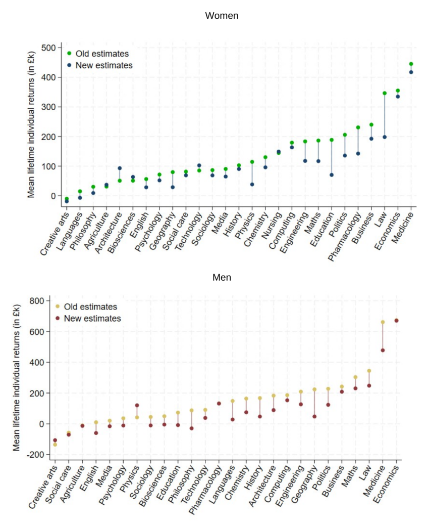
_{Note: ‘Old estimates’ are from Britton et al. (2020), in 2025/26 CPI prices. ‘New estimates’ are the main estimates from this report, and match the averages in Figures 5.6 and 5.7. Subjects are ordered by highest returns in Britton et al. (2020). Subjects for which HESA’s CAH2 codes have changed substantially between our old and new estimates are not shown. One exception that we do show is ‘Creative arts’, which is compared with ‘Creative and performing arts’ under HESA’s old classification.}

8. Returns by prior attainment

The expansion of higher education in England over recent decades has not been evenly distributed across the prior attainment distribution. Figure 8.1 shows the share of individuals participating in full-time undergraduate study by age 21 for various GCSE cohorts, separately for women and for men, by percentile of GCSE attainment within each cohort. At the top of the prior attainment distribution, participation rates were already very high amongst the 2002 cohort and have changed little since: students with the strongest GCSE results have always been very likely to attend university. The expansion has instead been concentrated amongst students with lower GCSE attainment. Amongst women in around the middle of the GCSE distribution, the share attending university by age 21 has risen by roughly 30 percentage points between the 2002 and 2018 GCSE cohorts. The pattern is similar for men, although participation rates amongst men remain lower than for women across the distribution.44

Figure 8.1. Share participating in full-time undergraduate higher education by age 21, by GCSE percentile for various GCSE cohorts

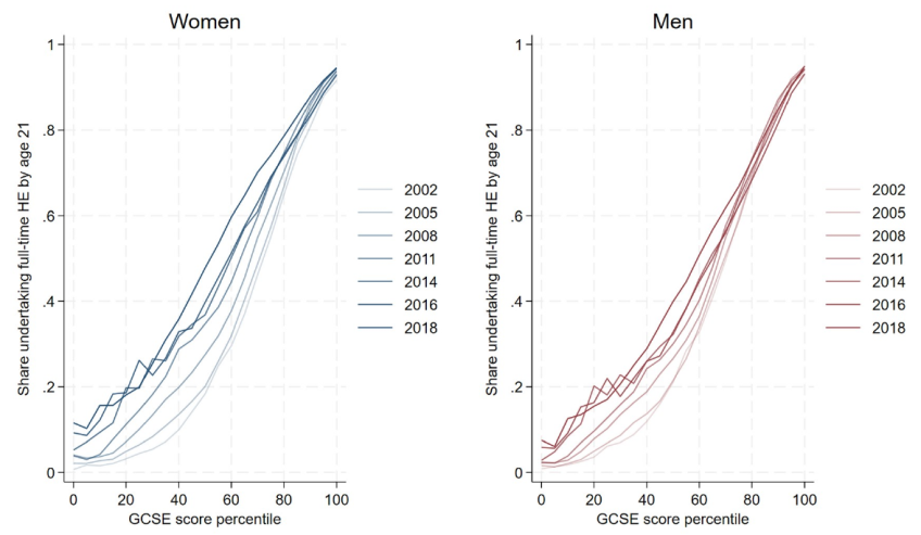
_{Note: Percentile rank of students’ point scores in their top eight GCSEs, rounded to the nearest 5. Includes full GCSE cohort in each year, without imposing sample restrictions around prior attainment or subject studied. Excludes students for whom we observe a master’s degree, PGCE or PhD but no undergraduate degree.}

This composition shift makes the returns to HE for students with lower prior attainment a question of first-order policy interest. An increasing share of new graduates are drawn from the lower part of the GCSE distribution, and the lifetime returns these students can expect are not necessarily well approximated by averages estimated across the full sample. In this chapter, we present estimates of lifetime returns specifically for the 35% of our analysis sample with the lowest prior attainment, again based on the 2002 GCSE cohort. We then present gross earnings returns at ages 28 and 35 by decile of prior attainment to provide suggestive evidence as to how returns may (or may not) vary between students at different points of the prior attainment distribution.

8.1 Net lifetime returns for ‘low prior attainment’ group

As discussed in Section 3.3, we define our ‘low prior attainment’ group as students who achieve at least the points equivalent of five C grades, but no more than four Bs and four Cs (or equivalent) in their top eight GCSEs. Figure 8.2 illustrates this definition by showing, for the 2002 GCSE cohort and within our analysis sample, the share of students attending each type of higher education institution (HEI) or not attending HE, by percentile of GCSE attainment. Our ‘low prior attainment’ group is indicated by the black box and corresponds approximately to the bottom 35% of the analysis sample. Both attending and not attending HE are common choices for this group: just over half (53%) of students in this group attended a full-time undergraduate course by age 21.45 Thus, for each HE student in this group, there are observably similar non-HE individuals to compare them with – meaning returns are well identified within this subgroup.

Figure 8.2. Proportion of students by institution type by percentile rank of GCSE scores, within 2002 GCSE cohort sample

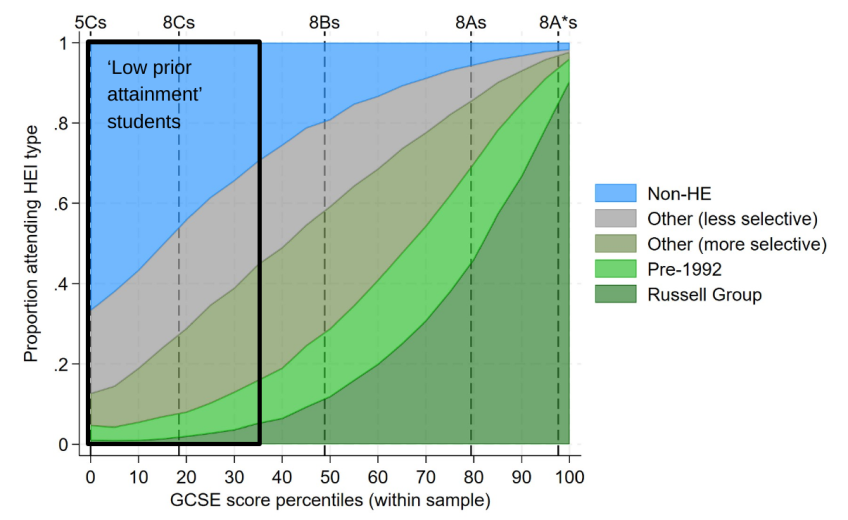
_{Note: Conditional on meeting sample restrictions, i.e. having a Key Stage 5 record and the points equivalent of five C grades in the student’s top eight GCSEs. Excludes part-time undergraduates, undergraduates beginning courses after age 21 and those attending other HE below undergraduate level. Dashed lines indicate percentile rank of students achieving points equivalent of five Cs (and no more), eight Cs, eight Bs, eight As or eight A*s in their top eight GCSEs. Percentile ranks are rounded to the nearest 5.}

It is worth noting that we do not capture the full set of academically marginal students within this ‘low prior attainment’ group. Of those in the 2002 GCSE cohort who are excluded from our analysis sample because they do not meet our GCSE points requirement or do not have a Key Stage 5 record, fewer than 5% started a full-time undergraduate course by age 21. Equivalently, of all students in the 2002 GCSE cohort who we observe starting a full-time undergraduate course by age 21, 92% are included in our main analysis sample. We are limited in what we can say about the individuals we do not capture: mostly likely, they have taken an unusual path through the school system, and their missing records are difficult to impute without biasing our overall estimates. There is also reason to think GCSE attainment is a noisier signal of underlying ability for these students than for those with more conventional school trajectories. While our estimates do not cover everyone, they do capture a large group of students for whom HE is far from a forgone conclusion.

Figure 8.3 shows median actual, counterfactual and simulated gross earnings by age for the ‘low prior attainment’ group, separately for women and for men. Two features are notable. First, the gap between median graduate earnings and median counterfactual non-HE earnings (for those who did attend HE) is narrower than in the equivalent figure for the full sample (Figure 5.1). This is most pronounced for men, where the gap between graduate and counterfactual earnings remains modest throughout the life cycle. Second, median earnings for ‘low prior attainment’ male graduates peak around age 50 and decline more sharply thereafter than for the full graduate sample, where median earnings remain higher for longer.

Figure 8.3. Median actual, simulated and counterfactual gross earnings by age for 2002 GCSE cohort: lowest-attaining 35% of our sample

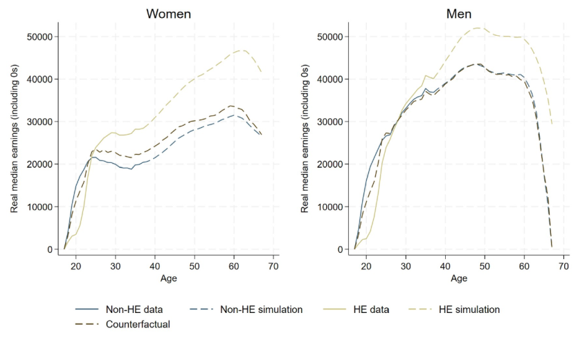
_{Note: ‘HE’ includes those who started a full-time undergraduate degree before the age of 21. Gross annual earnings in 2025/26 CPI prices. Includes zero earnings. Counterfactual earnings estimated as explained in Section 3.2. Sample selected as discussed in Section 2.1, including minimum GCSE attainment and a Key Stage 5 record. Data before age 27 exclude self-employment earnings. Earnings are uprated to reflect economy-wide real earnings growth between 2004/05 and 2023/24, and by 1.8% per year for every age after 37. Analysis restricted to students in approximately the bottom 35% of the sample according to GCSE scores, conditional on meeting the sample criteria.}

To estimate returns for this ‘low prior attainment’ group, we rerun our life-cycle simulations and regression analysis on the restricted sample as described in Section 3.3, dropping a small number of subject–institution cells with insufficient sample sizes within the subgroup. Counterfactual earnings predicted from background characteristics are also lower for this group than for the full sample, reflecting their lower average GCSE and Key Stage 5 attainment. This difference in counterfactual earnings – predicted earnings had those who attended HE not done so – is crucial in interpreting the returns estimates.

Table 8.1 presents our central estimates of net lifetime returns for the ‘low prior attainment’ group. Mean individual lifetime returns are £72,000 for women and £36,000 for men, compared with £90,000 and £109,000 for the full sample. Mean exchequer returns are £17,000 for women and £20,000 for men, well below the £48,000 and £107,000 estimated for the full sample.

Table 8.1. Average individual and exchequer lifetime returns, and share achieving positive returns, for women and for men: lowest-attaining 35% of our sample

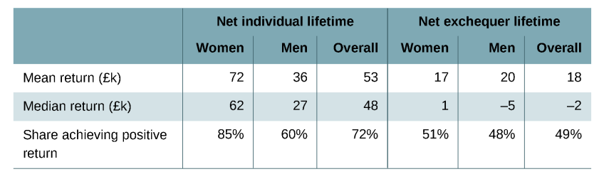
_{Note: All figures are shown in 2025/26 CPI prices and are discounted using Green Book discounting.}

One pattern that emerges clearly from these comparisons is that the gap between low-prior-attainment students and the full sample is much larger for men than for women. Mean individual returns for low-prior-attainment women are around 80% of those for the full sample of women, but for men the equivalent figure is around 33%. This partly reflects that the gender gap in returns reverses for this group: amongst the lowest-attaining 35%, mean lifetime individual returns are higher for women than for men, in contrast to the pattern in the full sample.46

The median individual returns are also lower for the ‘low prior attainment’ group than in the full sample, particularly for men – although the proportional reduction in median returns is smaller than for the mean returns. The median net individual lifetime return among the ‘low prior attainment’ group is £62,000 for women and £27,000 for men. These estimates are 93% and 45% of the full-sample estimates (of £67,000 and £60,000 respectively). This smaller reduction in the median returns is likely driven by a combination of there being fewer individuals within the ‘low prior attainment’ group achieving very high returns, and also the progressive nature of the tax and student loans systems.

The share achieving positive returns does not change as drastically as the means: 85% of women and 60% of men in the ‘low prior attainment’ group achieve positive individual returns, compared with 81% and 69% in the full sample. We estimate that the exchequer makes a positive return on approximately half of individuals in this group, down from around 60% in the full sample. We estimate that the exchequer approximately breaks even on the median woman in this subgroup, and makes a loss of around £5,000 on the median man.

Figure 8.4 shows cumulative average returns by age for the ‘low prior attainment’ group, both for individuals and for the exchequer. Returns turn positive later in the life cycle than for the full sample (Figure 5.4). With Green Book discounting, cumulative individual returns turn positive around age 30 for women and age 50 for men, compared with ages 27 and 38 respectively in the full sample. For low-prior-attainment men in particular, individual returns sit close to zero for a substantial portion of the life cycle.

Figure 8.4. Mean cumulative individual and exchequer returns to higher education by age: lowest-attaining 35% of our sample

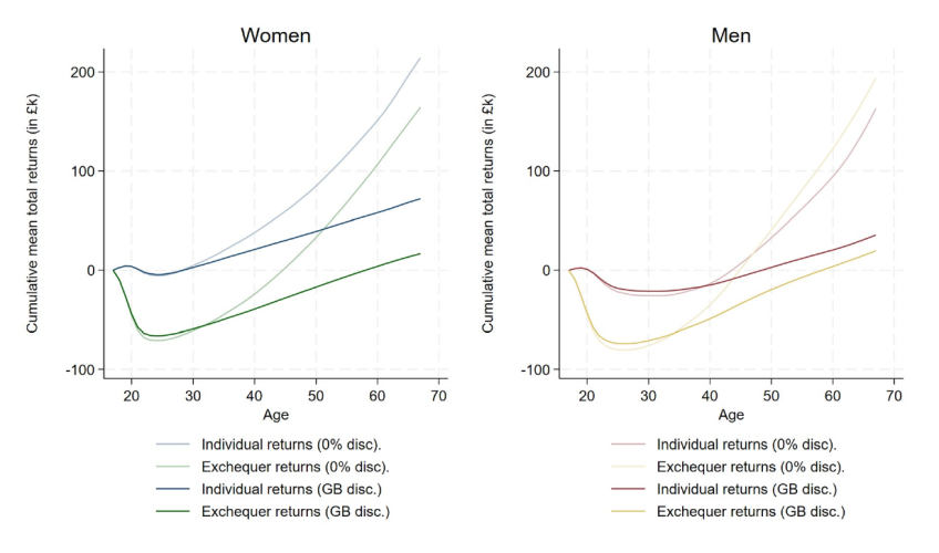
_{Note: All figures are shown in 2025/26 CPI prices and are discounted using either Green Book (GB) discounting, as in our main estimates, or with a 0% real discount rate. Returns at a given age are discounted cumulative returns to that age. Analysis restricted to students in approximately the bottom 35% of the sample according to GCSE scores, conditional on meeting the sample criteria.}

Figure 8.5 shows the distribution of lifetime net individual returns by subject, for women and for men, amongst the ‘low prior attainment’ group. Several subjects are excluded due to small sample sizes – notably, medicine (which is highly selective) for both men and women, and economics for women. Even setting these subjects aside, the estimates for nursing amongst women with low prior attainment are particularly striking. Nursing is the highest-return subject amongst these women, with mean returns of around £200,000 – well above business, computing and law. This likely reflects that nursing offers a reliable graduate premium through a regulated, structured-pay profession, making it a particularly strong proposition for women who would otherwise be lower in the earnings distribution. More broadly, the ordering of subjects is similar to that observed in the full sample (Figures 5.6 and 5.7): economics, business, computing and law remain amongst the highest-return subjects for men, while philosophy, creative and performing arts, and languages have low or negative average returns for both genders. For men, several subjects have negative average returns amongst the ‘low prior attainment’ group, including philosophy, creative and performing arts, English and languages.

Figure 8.5. Net lifetime individual returns to higher education by subject: lowest-attaining 35% of our sample

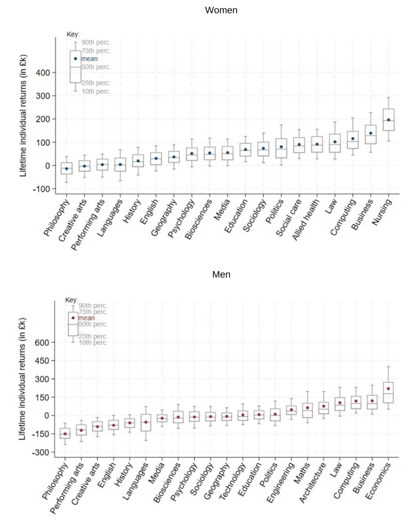
_{Note: All figures are shown in 2025/26 CPI prices and are discounted using Green Book discounting. Subject classification reflects CAH2. Subjects are ordered by mean average returns. Analysis restricted to approximately the bottom 35% of the sample according to GCSE scores, conditional on meeting the sample criteria. Subjects with low sample sizes within the ‘low prior attainment’ group are excluded. The ranges of the vertical axes differ between the panels.}

The strong correlation in subject ordering between the ‘low prior attainment’ group and the full sample partly reflects that, as discussed in Section 3.3, our simulation methodology applies common subject–age earnings growth profiles regardless of prior attainment. To the extent that low-prior-attainment graduates of a given subject would in fact experience slower earnings growth in their later careers than the average for that subject, our estimated returns for them will be modestly upward-biased. The fact that earnings already differ meaningfully for graduates and non-graduates with low prior attainment up to age 37 – as shown in Figure 8.3 – suggests that we are nonetheless capturing genuine differences in lifetime returns, even if the late-career earnings profiles are imperfectly tailored to this subgroup.

8.2 Gross earnings returns at ages 28 and 35 by prior attainment decile

In this section, we also estimate gross earnings returns at a given age within different prior attainment subgroups. This uses only the Longitudinal Education Outcomes data and avoids using late-career earnings simulations, which are less reliable in this context, given we cannot observe detailed measures of prior attainment in the Labour Force Survey data. This has the additional advantage that we can split our prior attainment subgroups more finely than for our lifetime estimates, presenting results by decile of prior attainment (within our main estimation sample) rather than only for the ‘low prior attainment’ group (the bottom 35th percentile).

Figure 8.6 presents the results from estimating equation (3.2) at ages 28 and 35. These are percentage annual earnings returns at a given age, controlling for the same rich background and prior attainment information from school records. They are gross earnings returns, i.e. without reflecting the up-front cost of higher education or applying the tax and student loans systems.

Figure 8.6. Gross earnings returns at ages 28 and 35 for students in 2002–04 GCSE cohorts, by within-sample prior attainment decile

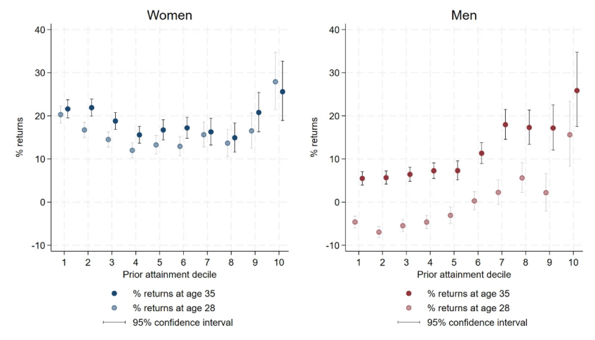
_{Note: See equation (3.2) in Section 3.3 for details of our regression model. Students are split into prior attainment deciles based on scores in their top eight GCSEs, within the selected sample after applying our sample selection criteria. These deciles therefore do not correspond to prior attainment deciles within the full GCSE cohort. Estimates are based on a pooled sample of students from the 2002, 2003 and 2004 GCSE cohorts and are conditional on observing positive earnings at the relevant age.}

Our results suggest that attending higher education is associated with higher gross earnings by age 35 throughout the distribution of prior attainment. Graduate women already see average gross earnings returns of 10–20 percentage points by age 28 across the prior attainment distribution (and closer to 30 percentage points for those with the highest prior attainment), and this changes little by age 35. For men, returns are much lower early on (and are slightly negative for those in the lowest prior attainment half) but continue to grow for longer. This is reflected by the much larger shift in returns between ages 28 and 35 than is visible for women. At age 35, we estimate gross earnings returns of between 5 and 10 percentage points for men in the bottom five deciles of prior attainment (the bottom half within our sample) and higher returns for those at the very top.

One striking pattern is that the relationship between returns and prior attainment differs between men and women. For men, there is a flat relationship in the bottom half of the prior attainment distribution and a positive relationship in the top half, at both ages. This results in the highest-attaining students seeing the largest returns, perhaps because they study the most competitive subjects and enter the most high-paying industries after graduating.47 In contrast, the returns follow more of a U-shape for women, with those at the bottom and top of the prior attainment distribution earning the highest percentage returns (although returns are higher in the highest prior attainment decile than in the lowest). At the top, this likely reflects similar subject and industry choices to those of higher-attaining men. At the bottom, it reflects very low earnings among low-prior-attainment women who do not attend HE.

9. How useful might these estimates be for more recent cohorts?

Our main estimates rely on lifetime earnings simulations for the 2002 GCSE cohort – the cohort for which we observe earnings for the longest, conditional on having detailed school records – and so reflect the labour market experiences of students who attended higher education in the mid 2000s. The returns for this cohort may not accurately reflect the returns for more recent cohorts, which – as we document below – look different in terms of the composition of prior attainment and in terms of subject–institution mix.

While we cannot estimate lifetime returns for today’s graduates as thoroughly as we can for the older cohorts, in this section we provide suggestive evidence on how the higher education landscape has changed since the 2002 GCSE cohort and the implications of those changes for returns for more recent cohorts. We begin in Section 9.1 by describing changes in who attends HE, including the subject and institution mix, drawing on HESA data up to the 2022/23 academic year. In Section 9.2, we consider what this compositional change might imply for average lifetime returns. We do this by reweighting our estimates for the 2002 cohort to reflect the subject and institution mix and background characteristics of 2022/23 university entrants. However, this relies on the assumption that the returns to a particular course for students with particular background characteristics have not changed – despite these compositional changes and the expanded supply of graduates – which is a particularly strong assumption. Section 9.3 therefore investigates directly whether gross earnings returns have changed for later cohorts of students. We examine estimates of how gross earnings returns at a given age have evolved, across up to 12 successive GCSE cohorts (2002–13) that we now observe up to at least age 26. This makes weaker assumptions than the analysis in Section 9.2 and so constitutes more robust evidence about the potential change in returns over time, but it cannot speak to the returns of the most recent HE attendees who we do not yet observe in the labour market.

9.1 Changes in who goes to higher education and what they study

Higher education has expanded dramatically in England over recent decades. Amongst the 2002 GCSE cohort, around 35% of women and 30% of men had started a full-time undergraduate degree by the age of 21 (Figure 9.1).48 For those who took their GCSEs in 2018, these proportions had risen to 53% and 40%, with a more pronounced increase amongst women. This is equivalent to an additional 87,000 students from the latest cohort participating in higher education compared with if the rate of participation had not changed.

Figure 9.1. Share of women and men in consecutive GCSE cohorts participating in full-time undergraduate higher education by age 21

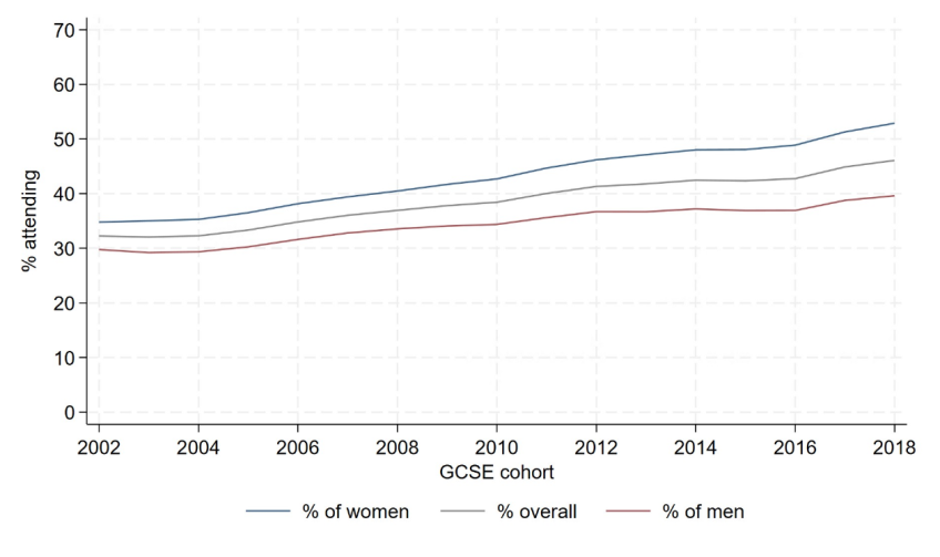
_{Note: Percentage of individuals in a given GCSE cohort who we observe starting a full-time undergraduate degree at a UK higher education provider by the age of 21, up to academic year 2023/24. A small number of students for whom we observe a master’s degree, PGCE or PhD but no lower-level degree are excluded from this chart and from the calculations in the paragraph above.}

This expansion has been spread unevenly across subjects. Some subjects have become increasingly popular over the last 15 years, including engineering, computing, business and economics among men, and nursing, medical sciences and sociology among women. There have been declines in the share of students studying some other subjects, including English, media and languages. These changes in subject choice are documented in Appendix K.

Broadly, a smaller share of university entrants are now studying subjects we estimated to have relatively low net lifetime returns (based on the estimated gross lifetime returns for the 2002 GCSE cohort) and a higher share of them are studying higher-return subjects. This is illustrated in Figure 9.2, which splits subjects into quintiles based on cash-terms estimated lifetime returns and shows the share of full-time undergraduate entrants studying each subject quintile over time. For men, there is a clear trend towards higher-return subjects, with the share studying subjects in the top quintile increasing from 27% in 2006 to 33% in 2021.49 This trend is slightly more muted for women, with an increase from 20% to 24% over the same years. That said, the trend reversed in 2022, with a jump in the share of students studying lower-return subjects.

Figure 9.2. Share of higher education students (those starting full-time undergraduate degrees by age 21) studying subjects in each quintile of average lifetime returns, by entry year

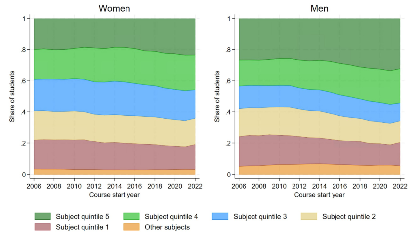
_{Note: Only includes individuals we observe with a Key Stage 4 record in LEO. We do not condition on any of our other sample restrictions (minimum GCSE scores, Key Stage 5 records or linked HMRC data). Subjects split into quintiles, separately by sex, by average net lifetime individual returns (according to Figures 5.6 and 5.7) weighted by number of students taking these subjects in our sample from the 2002 GCSE cohort. Quintile 5 represents the highest-return subjects and quintile 1 the lowest-return subjects. ‘Other subjects’ includes subjects for which we do not model lifetime returns (sport science, veterinary science, Celtic studies, and combined and general studies). Students studying joint degrees are weighted by full-person equivalents.}

The share of students attending each institution type has remained relatively stable over time. Figure 9.3 shows the share of full-time undergraduates in LEO who began their degrees by age 21 studying at each institution type. We use the same categories as in our lifetime earnings simulations for the 2002 GCSE cohort – even though some universities in the ‘other’ category may have become more or less selective in recent years. We also include an additional category for ‘not previously categorised’ universities. These either did not exist, did not have university status, or had too few students from the 2002–07 GCSE cohorts to be included.

Figure 9.3. Share of higher education students (those starting full-time undergraduate degrees by age 21) by institution type, by entry year

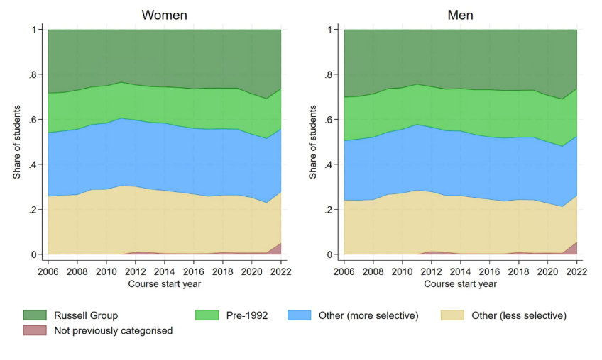
_{Note: Only includes individuals we observe with a Key Stage 4 record in LEO. We do not condition on any of our other sample restrictions (minimum GCSE scores, Key Stage 5 records, linked HMRC data or subject choice). Categorisation of universities into institution types is the same as that used for estimating lifetime returns for the 2002 GCSE cohort, with other universities split into more and less selective based on the average GCSE point scores of students from the 2002–07 GCSE cohorts attending these universities for full-time undergraduate degrees between ages 18 and 20. Universities with very small sample sizes were grouped with the ‘Other (more selective)’ universities for our lifetime estimates. Here we group them as ‘Not previously categorised’, alongside other universities that did not exist when the 2002–07 GCSE cohorts entered HE.}

Between 2006 and 2019, the intake shifted slightly towards less selective universities, and then back again. The share of female entrants at such universities started at 26% and increased to a high of 31% over this period, and the share of male entrants increased from 24% to 28% – though amongst both men and women these shares declined back to their 2006 levels by 2019. The share of students attending Russell Group universities followed the opposite trajectory: ranging from 28% in 2006 to 24% in 2011 and 26% in 2019 for women, and similarly from 30% in 2006 to 24% in 2011 and 27% in 2019 for men.

More recent years have seen a large shock to the university intake by institution type, with a large spike in students entering Russell Group universities in 2020 and 2021. Many university entrants in these years received teacher-assessed grades for their A levels due to exam disruption as a result of the COVID-19 pandemic, meaning they were more likely to meet their conditional offers at competitive universities. This was no longer the case in 2022, where instead we document a rise in undergraduates studying at universities that we previously had not classified.

9.2 Reweighting net lifetime returns to reflect today’s students

To provide suggestive evidence on what net lifetime returns might look like for more recent entrants, we can adjust our estimated average returns from Chapter 5 to reflect the characteristics of those who started university more recently.

In particular, we take our average net individual lifetime returns estimates – which reflect gross lifetime earnings returns for the 2002 GCSE cohort – and reweight them, separately by sex, to reflect changes in the shares studying each subject and at each of our four institution types up to the 2022/23 university entry cohort, which is the most recent year we can look at using our data. Within each sex–subject–institution-type cell, we match individuals from the 2022 entry cohort to those from the 2002 GCSE cohort who were most similar to them in terms of prior attainment and proxies for socio-economic status (IDACI and an exact match on whether they attended a private school) and assign them the same net lifetime return as their closest neighbour.50

This exercise may provide some suggestive evidence as to how average lifetime returns may have changed for later cohorts given only changes in the subject and institution mix and background characteristics of those entering higher education over time. However, this requires the strong assumption that subject- and institution-specific lifetime returns have not changed over time. We will not be reflecting changes in returns within these cells – for example, as a result of changes in labour market conditions, an increase in the supply of graduates or other features of the graduate experience. It also relies on an assumption that, within each sex–subject–institution-type cell, the relationship between prior attainment, socio-economic status and lifetime earnings returns has not changed across the two cohorts. We cannot test either of these assumptions directly for the 2022 entry cohort, although we are somewhat reassured by analysis of returns at specific ages which suggests similar assumptions may have been reasonable when comparing successive GCSE cohorts and that the relationships between background characteristics and earnings have been fairly stable over time (Section 9.3).

As shown in Table 9.1, reweighting actually increases our headline estimated average return for women, from £90,000 to £104,000, and leaves the estimate for men largely unchanged at £110,000. This is despite increases in the share of students entering HE who are from groups that typically have lower returns on average in cash terms: those who were not at a private school at age 15, who were living in relatively more deprived areas and who had lower prior attainment.

Table 9.1. Average net individual lifetime returns, and share achieving positive returns, for women and for men

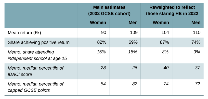
_{Note: All figures are shown in 2025/26 CPI prices and are discounted using Green Book discounting. Median returns figures are not presented as it is not clear they are meaningful given how the reweighting is performed. Median percentiles are median percentile ranks of those attending HE by age 21, in each case computed within full GCSE cohorts. A higher IDACI score is associated with higher relative area deprivation.}

As shown in Figure 9.4, the impact of these changes on the overall reweighted averages has been offset by changes in the subject mix. Amongst women, there has been a slight shift towards studying subjects that were associated with higher gross earnings returns for women in the 2002 GCSE cohort, but additionally reweighting for any changes in institution type makes little further difference, consistent with the evidence in Section 5.2 that average net lifetime returns are similar across university types for women. There has been a more significant shift towards studying subjects that we estimate were higher-return for the 2002 GCSE cohort amongst men, but the impact on the reweighted return is offset by a slight shift towards less selective universities – which are associated with lower returns amongst men – and a clearer shift within subject–institution-type cells and towards background characteristics associated with lower returns.

Figure 9.4. Decomposition of changes in average net individual lifetime returns if reweighted to reflect 2022 university entry cohort

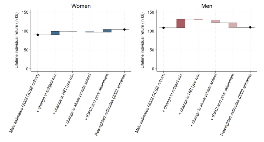
_{Note: Mean average returns amongst sample in sex–subject–institution-type combinations that exist in sufficient sample sizes amongst those who enter full-time undergraduate higher education by age 21 both in the 2002 GCSE cohort and the 2022 university entry cohort. Overall averages for 2002 cohort do not precisely match returns for the main analysis sample presented in Table 5.2.}

While only illustrative, this reweighting exercise at least does not provide strong evidence that lifetime returns are likely to be lower on average as a result of changes in who goes to higher education and what they study.

9.3 Changes in estimated gross earnings returns for later cohorts

Relative to our previous report, we now have additional years of earnings for existing cohorts, as well as fully linked LEO data for later birth cohorts. This means we can attempt to look at how earnings returns may have changed across cohorts.

We provide descriptive evidence as to the early labour market experiences of later cohorts in Appendix L and we show how raw earnings gaps between graduates and non-graduates have changed over time in Appendix M. Once we focus on only those who had a realistic option of attending higher education based on their prior attainment, the earnings trajectories of young graduates and non-graduates look strikingly similar across the 14 GCSE cohorts since 2002. Raw earnings gaps between graduates and non-graduates at a given age are flat over time (across consecutive cohorts), despite a large increase in HE participation over this period. For neither men nor women do we see any compelling evidence that raw earnings gaps at specific ages have changed substantially between successive cohorts.

Estimated gross earnings returns at specific ages

In this subsection, we investigate whether the gross earnings returns to HE at specific ages appear to have changed over successive cohorts. To do this, we estimate equation (3.3) separately by sex, age and cohort, following the methodology in Section 3.4.51 We exclude students who do not meet a minimum level of attainment or who are missing background characteristics, and so again focus on only those for whom attending HE was a realistic option given their prior attainment. We control for a rich set of background characteristics, and so consider the differences in earnings of graduates and non-graduates (from the same cohort, at the same age) that cannot be explained by differences in the observable characteristics of those graduates and non-graduates. We focus on the 12 GCSE cohorts for which we observe earnings in the tax data up to at least age 26.

We present our results in Figure 9.5. Each line representing percentage returns at a given age is approximately flat, implying there has not been a systematic increase or decrease in the returns over successive cohorts.52 The relationship between age and returns is positive for men but concave for women. For instance, for the 2002 GCSE cohort, we estimate returns of 22% at age 26 for women, which increase to 29% at age 29, before falling back to around 22% at ages 35 to 37. This is similar to the patterns in the raw earnings gaps shown in Figure M.2 in Appendix M.

Figure 9.5. Gross earnings returns at ages 26 to 37 for consecutive GCSE cohorts

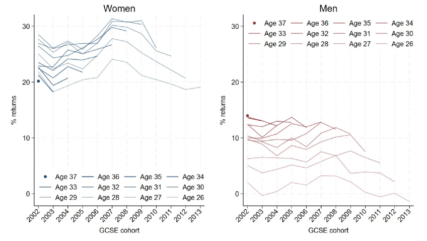
_{Note: Results are based on estimates of equation (3.3) following the methodology discussed in Section 3.4. Figures are conditional on positive earnings at the relevant age. Earnings at age 26 for 2002 GCSE cohort exclude self-employment earnings.}

One clear result from comparing these estimates of returns with the raw earnings gaps in Appendix M is that our estimates of returns remain much lower than the raw earnings gaps. As for the 2002 GCSE cohort, differences in background characteristics continue to account for a large share of gaps in raw earnings between graduates and non-graduates when we look at later cohorts. Figure 9.6 makes this point more explicitly by showing the role of background characteristics in explaining returns at age 28 for successive cohorts. We estimate that the share of the earnings gap explained by differences in background characteristics is reasonably stable at around £3,000–4,000 in today’s prices across all cohorts we observe at this age. This selection effect accounts for 35–40% of the raw earnings gap for women and 60–65% of the gap for men. The remaining returns are a relatively constant wedge above this selection effect, and once again we do not find evidence that returns have declined amongst later GCSE cohorts.

Figure 9.6. Average gross earnings of HE and non-HE groups at age 28 for consecutive GCSE cohorts

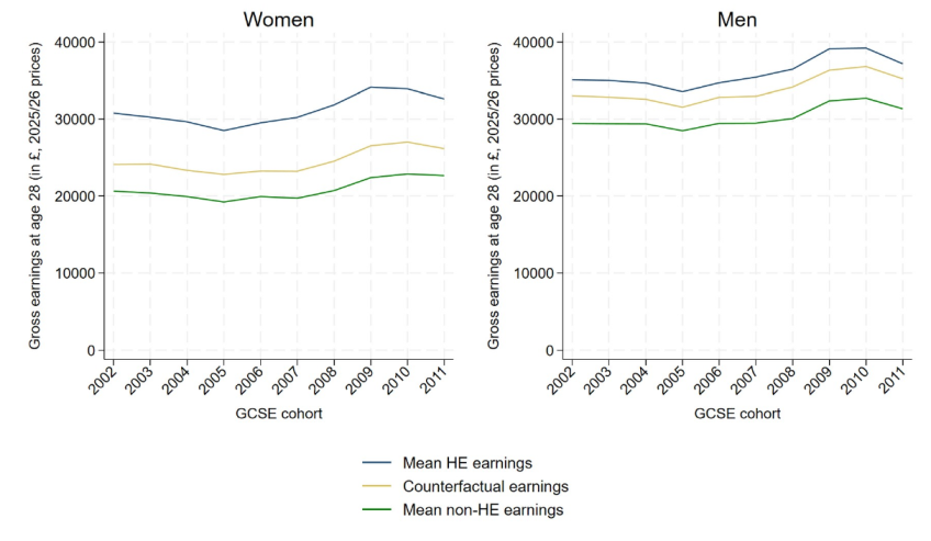
_{Note: Results are based on estimates of equation (3.3) following the methodology discussed in Section 3.4. Figures are conditional on positive earnings at age 28. ‘HE’ and ‘non-HE’ groups are as defined in Section 2.1. Counterfactual earnings reflect predicted earnings of the HE group had they not attended HE, based on their background characteristics and prior attainment. The difference between counterfactual and HE earnings at each age corresponds to the % gross earnings returns at age 28 shown on Figure 9.5.}

It is worth clarifying at this point that this result – that gross earnings returns have been stable across cohorts – is distinct from our earlier finding in Chapter 7 that we now estimate average net lifetime returns for a single cohort to be lower than in Britton et al. (2020). There need not be any tension between these findings: we now expect the 2002 GCSE cohort to experience lower gross earnings returns over their lifetimes than we estimated for that same cohort in earlier work, and we now apply a different set of government tax and student loan policies to estimate net lifetime returns. We do not find evidence that those from later cohorts have experienced lower gross earnings returns than that 2002 cohort did early in their careers.

Comparison with other evidence on the changing graduate premium

Existing research has produced a mix of results on how the UK’s graduate premium has changed over time, with some arguing it has declined. For example, Stansbury, Turner and Balls (2023) find that the graduate hourly wage premium decreased in all regions of the UK between 1997 and 2019 (outside London), while Boero et al. (2025) estimate that the annual graduate earnings premium at age 26 decreased by around 10 percentage points between the mid 2000s and the late 2010s. On the other hand, Blundell, Green and Jin (2022) find that the UK’s graduate premium remained relatively flat between 1993 and 2016, at least across birth cohorts from the 1960s to the 1980s – earlier cohorts than we are able to examine using the LEO data.

Our analysis shows that subtle differences in how the graduate premium is calculated can lead to substantial changes in the conclusions. Most obviously, when we restrict the sample to individuals with a minimum level of GCSE attainment in Figure M.2, this eradicates any decline in the raw graduate earnings premium seen over successive cohorts in Figure M.1. This may imply that reported declines in the graduate premium are driven partly by economic changes such as increases in the minimum wage which predominantly affect lower-attaining non-graduates who did not continue in education beyond age 16. When estimating the returns to undergraduate degrees for those who started them, such non-graduates are a less relevant comparison group.

More generally, there are a number of potential reasons for the differences between our estimates and others’: differences in data sources, age ranges, sample restrictions, control variables, and whether the outcome is annual or hourly earnings. We use detailed administrative data, apply a minimum-attainment sample restriction (to compare only with non-graduates who could plausibly have attended HE), and estimate earnings returns controlling for a very rich set of background characteristics separately by age and cohort. Using administrative data in particular means we have much larger sample sizes and potentially more reliable measures of earnings (from tax records rather than self-reports). Work that has relied on survey data, such as from the Labour Force Survey, has typically considered hourly earnings, examined a longer period of time, and pooled across multiple ages and cohorts. Previous work (e.g. Stansbury, Turner and Balls, 2023) has also documented geographical variation in changes to the graduate premium over time; that is beyond the scope of our report.

Estimated gross earnings returns at age 28 by subject

Finally, we examine whether returns by subject have changed over time. To do this, we estimate the same model as used elsewhere in this chapter, but with multiple dummies for each university subject in place of a single HE dummy. We present gross earnings returns by subject at age 28 for 10 consecutive GCSE cohorts in Figure 9.7. Two points are worth noting. First, our estimates are subject to uncertainty and the range of returns to each subject is reasonably wide over 10 cohorts. Second, the broad ranking of subjects does not change much between cohorts: subjects that were relatively low- or high-return for the 2002 GCSE cohort at age 28 (in 2014/15) tended to be the same subjects that were relatively low- or high-return for the 2011 GCSE cohort at age 28 (in 2023/24).

Figure 9.7. Gross earnings returns at age 28 for consecutive GCSE cohorts, by subject

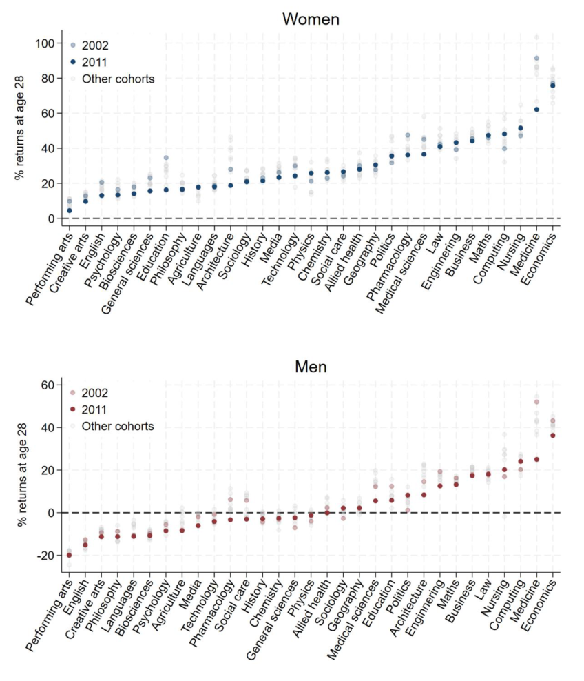
_{Note: Results are based on estimates of equation (3.3) following the methodology discussed in Section 3.4, but with dummy variables for whether an individual studied each subject in place of a single HE dummy. Figures are conditional on positive earnings at the relevant age. The subject classification reflects CAH2 and excludes a small number of subjects due to low sample sizes. Each dot represents a separate GCSE cohort. Subjects are ordered by mean average returns for the 2011 GCSE cohort.}

There are some notable exceptions to this. In particular, we estimate a large decrease in earnings returns at age 28 amongst those who studied education, medicine and pharmacology degrees when looking at later GCSE cohorts. This may reflect that many graduates from these courses will have entered public sector professions where recent real earnings growth has been slow or non-existent.53 The same declines have not been seen for nursing graduates.

Taking all the results in this section together, we do not find evidence that returns to attending higher education have changed substantially over time, either overall or by individual subject area, at least amongst people for whom attending HE was a realistic option.

10. Conclusion

We estimate that the average undergraduate degree in England is a financially worthwhile investment for both individuals and the taxpayer. We estimate large gross lifetime earnings returns to attending university for individuals who took their GCSEs in 2002: they can expect to earn substantially more on average over their working lives than if they had not attended university. When we apply the current tax and student loans systems – which are likely to be of more interest to policymakers and prospective students than the policies that applied for the 2002 cohort – we estimate mean individual lifetime returns are around £90,000 for women and £109,000 for men in 2025/26 prices, and mean exchequer returns are approximately £48,000 and £107,000 respectively. The vast majority of graduates – 81% of women and 69% of men – can expect to be better off financially than a similar young person who did not go to university, even after accounting for extra income tax, employee National Insurance contributions and student loan repayments.

These estimates are nonetheless lower than those in our previous report (Britton et al., 2020). The most important reason is that actual earnings for the 2002 GCSE cohort have come in below what the 2020 estimates anticipated – especially for graduates – reflecting weak real earnings growth across the economy over the past decade. This should not be read as evidence that the value of higher education is declining over time, only that we now estimate the gross lifetime earnings return for this specific cohort to be lower than we did in previous work. Indeed, we find that the percentage gross earnings return (the difference between the earnings of graduates and non-graduates with the same background characteristics) at given ages has been remarkably stable across the next 11 GCSE cohorts. We do not find any evidence that the earnings returns to attending university have markedly worsened for more recent cohorts, at least early in their careers.

Tax and student loan policy changes between 2019/20 and 2025/26 have also shifted the balance between individual and exchequer returns. Frozen tax thresholds, less generous maintenance loans, and tighter student loan repayment terms have all reduced individual returns and increased exchequer returns. Strikingly, despite the worse picture for underlying gross earnings returns, estimated mean exchequer returns for women are now higher than in our 2020 estimates (reductions to tuition fees and teaching grants in real terms also contributed to higher exchequer returns).

Variation around these averages remains very large. Returns differ substantially by subject and, especially for men, by institution: several subjects show low or negative returns on average (although this does not imply that all students of these subjects will achieve negative returns).

Students with lower prior attainment see lower net lifetime returns than the full sample in cash terms, particularly men, although mean returns are still positive both for individuals and for the taxpayer. For this group, however, returns turn positive later in the life cycle, and we estimate that the exchequer makes a positive return on only around half of these students. When we consider returns across all deciles of prior attainment, we estimate average gross earnings returns are positive at age 35 across all levels of prior attainment.

We also investigate returns based on the composition of students entering higher education today. Today’s students have lower average prior attainment than in the 2002 GCSE cohort, which would tend to push down average returns. But this has been largely offset by a shift towards higher-return subjects – particularly among men. Reweighting our main estimates to reflect the characteristics and subject mix of the 2022 university entry cohort suggests that average returns may, if anything, be slightly higher today than for the 2002 GCSE cohort, although this conclusion rests on the strong assumption that returns within subject–institution–background cells have not changed.

Our results should be interpreted with the caveats inherent in projecting lifetime earnings returns based on data from cohorts that entered higher education around 20 years ago. Available evidence suggests that the earnings of the 2002 GCSE cohort are informative for policymakers and students today, and we apply today’s tuition fee, student loan and tax policies to make our net returns estimates more relevant to current students and policymakers. But it is not possible to predict with certainty how much current students will earn over the next five decades, or how much they would have earned if they had not gone to university. Significant changes in the structure of the labour market, in the nature of graduate work or in the policy environment could change these conclusions for future cohorts of students. Again, we note that this report covers financial returns only; broader non-pecuniary returns to higher education and potential spillovers to others are outside its scope, as is the question of what is the optimal level of participation or investment (public or private) in higher education.

Appendices

Appendix A. Data and sample selection

This appendix describes the data we use more precisely, as well as the sample selection criteria we apply to arrive at our main analysis sample. It explains how we categorise individuals into our higher education (HE) and non-HE groups, describes the subject classification used (and which degree subjects are dropped) and provides details of the matched HESA–HMRC data we use and the Labour Force Survey (LFS).

Longitudinal Education Outcomes (LEO)

We use the Longitudinal Education Outcomes (LEO) dataset, which links labour market outcomes to school, further education and higher education records, as described in Chapter 2.

We restrict our main analysis sample (‘2002 GCSE cohort’) to individuals who:

• Attended a school in England in the year in which they took their GCSEs.
• Have non-missing key variables in the National Pupil Database (with an exception for independent school students not covered by the School Census, for whom missingness would be expected by construction).
• Did not attend a special school specifically for children with SEND, and did not have a SEN statement or EHCP at age 16.
• Achieved at least the points equivalent of five C grades in their top eight GCSE exams.
• Have a Key Stage 5 (KS5) record within three years of the year in which they sat their GCSEs.
• Either started a full-time first undergraduate degree course by the age of 21 or had not started any higher education course by age 37. This excludes those studying an undergraduate degree part-time or starting between ages 22 and 37, and those whose only higher education course was at below undergraduate level.
• Did not study courses in some specific subjects where sample sizes are too small to draw reliable conclusions about lifetime earnings – in particular, sport science, veterinary science, Celtic studies, and combined and general studies.
• Can be successfully linked to a tax record in HMRC data and who are observed to have non-zero earnings in at least one tax year.

These restrictions reduce our sample size from around 590,000 students who took a GCSE exam in the 2001/02 academic year to 209,131 in our main analysis sample, as shown in Table A.1. This reduction is predominantly driven by sample restrictions which limit our focus to those who could plausibly have attended higher education by age 21. Match rates within the administrative data are extremely good. Of those observed attending a school in England in the year in which they took their GCSEs, 98.5% are either matched to a record in the School Census or attended an independent school. We observe non-missing GCSE grades for nearly all of these students, and most (91%) can be matched to an earnings record in the tax data. A large majority can also be matched to Key Stage 2 attainment data, although we do not require this for our sample criteria.

Table A.1. Analysis sample (2002 GCSE cohort) as sample restrictions added in turn, by sex

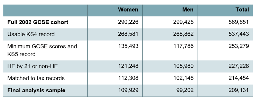
_{Note: Number of individuals in our sample, including HE and non-HE groups, as sample restrictions added in turn. Note that the ‘Full 2002 GCSE cohort’ line may overstate the number of pupils actually in that GCSE cohort because some people taking exams a year early appear in the Key Stage 4 attainment records. These account for over half of the individuals dropped in the next line. ‘Usable KS4 record’ excludes students who are missing important background information from the School Census (unless they attended an independent school), who have a SEN statement or EHCP or attended a special school, or who we associate with a different GCSE cohort. ‘Minimum GCSE scores and KS5 record’ conditions on achieving at least the points equivalent of five C grades in their top eight GCSEs, and on having a Key Stage 5 record within three years of the Key Stage 4 record. ‘HE by 21 or non-HE’ excludes part-time undergraduates, students beginning a degree for the first time between ages 22 and 37, and students whose only higher education course was at below undergraduate level. ‘Matched to tax records’ conditions on a successful link to HMRC data and positive earnings being observed in at least one year, excluding those who have, for instance, died or permanently emigrated. ‘Final analysis sample’ excludes a few subjects for which we do not model lifetime returns.}

We split higher education institutions into the following categories:

• Russell Group universities;
• old (pre-1992) universities not in the Russell Group;
• other universities, split into more and less selective categories based on the average GCSE point scores of those attending these universities for full-time undergraduate degrees beginning between ages 18 and 20 from the 2002–07 GCSE cohorts.

These are very similar to the categories used in Britton et al. (2020), although we now use more years of data to estimate the relative selectivity of other universities, leading to six universities switching between the more and less selective categories. A full list of providers by institution type is provided in Appendix N. Table A.2 presents the number of students in the 2002 GCSE cohort used in our main analysis by institution type, with those not attending higher education included as another category.

Table A.2. Analysis sample (2002 GCSE cohort) by institution type and sex

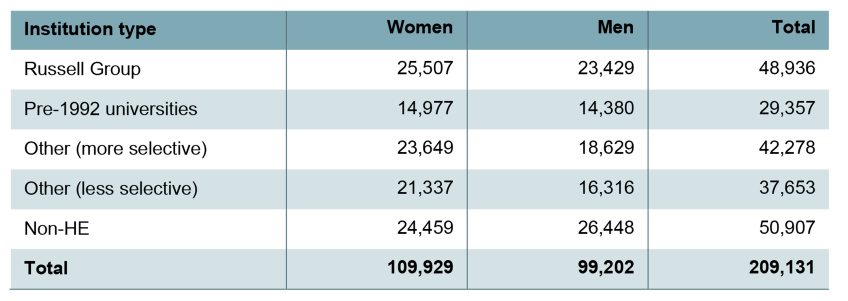
_{Note: Number of individuals attending each institution type in our sample, as well as those not attending HE, from the 2002 GCSE cohort. ‘Non-HE’ conditions on having the points equivalent of five C grades in their top eight GCSE exams and a Key Stage 5 record and excludes those with other HE trajectories. The ‘other’ category is split into more and less selective universities based on the average GCSE point scores of those attending these universities for full-time undergraduate degrees beginning between ages 18 and 20, from the 2002–07 GCSE cohorts. Universities with very low sample sizes are grouped with the more selective universities.}

To estimate and report returns by subject area, we use the second level of HESA’s Common Aggregation Hierarchy (hereafter CAH2), which contains 35 subject categories. We follow the most recent version of the classification (version 1.3), although note this means some results at the subject level will not be fully comparable to results from Britton et al. (2020), who used an earlier version of the CAH2. As in the 2020 report, we exclude four subjects – sport science, veterinary science, Celtic studies, and combined and general studies – due to low sample sizes in either the LEO or LFS data for the relevant cohort. We also do not present results for male nursing graduates, though we include them in our sample. Sample sizes by subject area are reported in Table A.3.

Table A.3. Analysis sample (2002 GCSE cohort) by subject area and sex

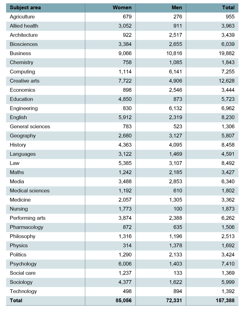
_{Note: Number of individuals attending HE in our sample, by subject area at CAH2. In full-person equivalents (FPE), weighted by share of time spent studying each subject. Total number of FPE students in these subject areas (157,388) is slightly lower than the total number of individuals in our HE group (158,224) as some spend some share of their time studying other subject areas. Totals may not sum due to rounding.}

Where individuals are studying courses across multiple subject areas, they are included in multiple subjects, weighted based on the nominal share of their time apportioned to each subject area (xfpe01).

For the analysis of returns amongst those in a ‘low prior attainment’ group in Chapter 8, we further restrict the sample to those in approximately the bottom 35% of our analysis sample by GCSE attainment. These students achieve at least the points equivalent of five C grades but no more than four Bs and four Cs (or equivalent) in their top eight GCSEs. Compared with our full sample, a much higher share of students with low prior attainment are in our ‘non-HE’ group, and the share attending Russell Group or other pre-1992 universities is much lower (see Table A.4).

Table A.4. Analysis sample (2002 GCSE cohort) by institution type and sex for the ‘low prior attainment’ group

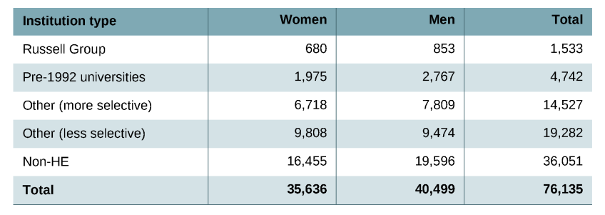
_{Note: Conditional on meeting sample restrictions, i.e. having a Key Stage 5 record and the points equivalent of at least five C grades but no more than the equivalent of four Bs and four Cs in their top eight GCSEs.}

HESA–HMRC

For our HE group, we also use additional administrative data: linked Higher Education Statistics Agency (HESA) and HM Revenue & Customs (HMRC) records for students from the 1978/79 to 1984/85 birth cohorts. For these students, we observe degree subject and institution attended, as well as earnings and employment from tax records. These cohorts are not linked to the National Pupil Database, so we cannot exclude students based on their prior academic attainment. We restrict the data to England-domiciled students who start full-time undergraduate degrees between ages 17 and 21 and exclude the same list of subjects with small sample sizes as above. Table A.5 shows sample sizes from the HESA–HMRC data by cohort and sex. The match rates – and hence the sample sizes – increase for later birth cohorts.

Table A.5. Analysis sample from HESA–HMRC data by birth cohort and sex

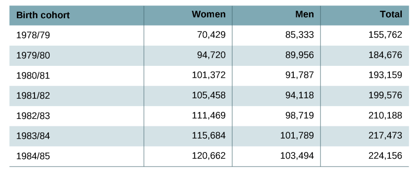
_{Note: Includes only England-domiciled undergraduates studying full-time undergraduate degrees beginning before age 21, who are matched to HMRC records and are studying subjects for which we model lifetime returns. We cannot apply sample criteria based on prior attainment as these cohorts are not linked to the National Pupil Database.}

Labour Force Survey (LFS)

To simulate earnings beyond age 37 for our cohort of interest, we use data from the Labour Force Survey (LFS), a quarterly household survey. As described in Chapter 2, we derive two datasets from the LFS: a five-quarterly LFS panel, linking individuals’ responses from waves 1 and 5, and a repeated cross-section of earnings for a larger sample of individuals. In each case, we restrict our LFS analysis sample to individuals who:

• Had their highest qualification achieved as either GCSEs or A levels (or equivalent), or a full degree, i.e. dropping those with highest qualification achieved below GCSEs or HE below degree level (hiquald).
• For those with GCSEs or equivalent as their highest qualification, had at least five passes at A*–C in O levels, GCSEs or equivalent (numol5).
• Reported their country of birth as being in the UK (cry12). We do not observe whether individuals were specifically born in England in some survey waves.
• Were aged between 25 and 59 when surveyed. We use data from ages 25 to 36 to smooth our parameters over a wider range of ages, but for our main analysis we rely only on ages 37 to 59.
• Had non-missing earnings information. This excludes self-employed individuals.

For those in our HE group, we map their reported degree subject (sngdeg, fdsngdeg) onto the CAH2 classification version 1.3.

We use LFS data from 1997 up to March 2020 for our earnings profiles. For the copulas, probits and earnings ranks of individuals re-entering employment, we use estimates from Britton et al. (2020) which relied on LFS data up to 2018. We report unweighted sample sizes for the repeated cross-section between ages 37 and 59 in Table A.6. We aggregate at the level of subject group and sex for presentational purposes.

Table A.6. Analysis sample from Labour Force Survey by subject group and sex

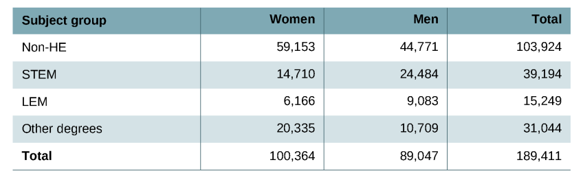
_{Note: Sample size for our repeated cross-section of individuals aged 37–59 appearing in the LFS between 1997 and 2020. STEM stands for science, technology, engineering and maths. LEM stands for law, economics and management.}

Appendix B. Further detail on methodology

Discounting

The formula for converting an individual’s earnings stream between the ages of 17 and 67 ${\left\{y_{i,a}\right\}}_{17}^{67}$ into a lifetime earnings figure is

$$Y_i=\sum _{a=17}^{67}\frac{y_{i,a}}{{\left(1+d\right)}^{a-17}}$$

where $y_{i,a}$ is an individual’s earnings at a given age and $d$ is the discount rate. A discount rate above 0 implies that income earned in the future is worth less than income earned today, with the degree of ‘impatience’ increasing in $d$. A discount rate of 0 assigns the same weight to all income regardless of the age at which it is earned.

For our main estimates, we apply Green Book discounting and express lifetime returns in terms of earnings at age 18. This means we do not discount earnings at age 17 or 18, we discount earnings by 3.5% for the next 30 years, and then by 3.0% thereafter. Hence, the precise discounting formula for our main estimates is

$$Y_i=y_{i,17}+\sum _{a=18}^{48}\frac{y_{i,a}}{{1.035}^{a-18}}+\sum _{a=49}^{67}\frac{y_{i,a}}{{1.035}^{30}\times {1.03}^{a-48}}$$

This implies that income earned at age 18 is 4.92 times as valuable as income earned at age 67 for calculating lifetime earnings.

Student loan outlay

We assume all students are charged the maximum tuition fee cap for standard full-time courses at providers with a TEF (Teaching Excellence Framework) award and an APP (Access and Participation Plan). This is £9,535 in 2025/26, £9,790 in 2026/27 and £10,050 in 2027/28, and is thereafter assumed to increase each year in line with forecast RPI (Retail Prices Index) inflation, in line with current government policy. We assume that all students take out a tuition fee loan to cover the full value of their fees and that they borrow the maximum they are entitled to towards their living costs in each year that they study.

We approximately match maintenance loan entitlements in the 2025/26 academic year and assume that these entitlements increase in each subsequent academic year in line with forecast CPI (Consumer Prices Index) inflation. We account for lower maintenance loan entitlements for final year students and we reflect rules that limit borrowing to the expected length of a student’s course plus one year.

How much students are eligible to borrow for their living costs (their maintenance loan entitlement) depends on whether they study at a university in London and whether they are living at home (typically with their parents). We observe the former in the LEO data and randomly assign the latter to match the proportion of recent accepted applicants who intend to live at home while studying. For this, we use the proportion of England-domiciled accepted applicants through UCAS, aged 17–20, who reported that they intended to live at home while studying, which was 32% in 2025 (UCAS, 2025).

Maintenance loan entitlements also reflect household residual income (HHRI), with those from lower-income households eligible to borrow the maximum. Given we do not observe actual household income in the data, we divide our HE sample into three groups based on socio-economic background variables available in the administrative data (specifically, neighbourhood deprivation and whether they attended a private school). We assume the most disadvantaged 49% are eligible for the maximum support, the most advantaged 34% are eligible for the minimum, and the remainder are eligible for the mid-point between the minimum and maximum. Among English, Welsh and Northern Irish first undergraduate degree entrants in the 2023/24 academic year, 42% reported an HHRI of between zero and £25,000 and 48% reported an HHRI of at least £42,601 or were non-responders (Office for Students, 2025a). It is not possible to compare with England-domiciled students only based on published statistics, but this suggests we may be slightly overestimating maintenance loan entitlements of more recent starters – particularly as HHRI thresholds have remained frozen in cash terms since 2023/24.

Together, we estimate average loan outlay of £53,500 with Green Book (GB) discounting, of which £29,700 is for tuition and £23,900 for maintenance. With 0% real discounting, which is more comparable to forecasts of loan outlay published by DfE, we estimate average loan outlay of £56,700 (Table B.1). This is higher than DfE’s official estimate of mean average total loan amount per borrower starting in the 2025/26 academic year, which was £45,900 amongst all higher education full-time borrowers (Department for Education, 2025a). We expect this difference largely reflects that we assume graduates take up their maximum loan entitlement each year: in practice, they may borrow only some of the amount they are entitled to, or for only some years of study. (Those who do not borrow at all will be excluded from DfE’s estimates, which relate to student loan borrowers only.)

Table B.1. Estimated average loan outlay by completed years of study

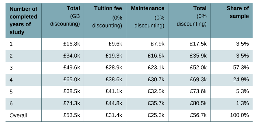
_{Note: All figures are shown in 2025/26 CPI prices and are discounted using either Green Book (GB) discounting, as in our main estimates, or with a 0% real discount rate. Share of sample reflects share of our main estimation sample (the HE group from the 2002 GCSE cohort) in each row, and may not sum as a small number of students are observed to participate for parts of some years, or for more than six years; these students are included in the ‘Overall’ average.}

For those we observe studying and model as taking up support for three years (the length of a typical undergraduate degree), our estimated loan outlay (£52,000 with 0% real discounting) is much more similar to DfE’s estimate for those who actually borrow for three years (£49,300). Indeed, our estimates of mean tuition fee and maintenance loan outlay amongst those we assume take up loan funding for one year (£9,600 and £7,900) are very similar to DfE estimates of average loan outlay per full-time undergraduate borrower in the 2025/26 academic year (£9,100 and £8,000).

Student loan repayments

Our main estimates apply the ‘Plan 5’ student loan terms faced by those beginning undergraduate degrees in 2025/26. Under this system, graduates pay back 9% of earnings above £25,000. This threshold is set to be frozen until April 2027, after which we assume it increases each year with forecast RPI inflation, in line with current government policy. We model the application of interest to loan balances at RPI, and assume repayments stop at the end of the write-off period, 40 years after graduation. We assume no borrowers make voluntary repayments.

In Chapter 6, we show the sensitivity of our results to instead assuming that graduates were subject to ‘Plan 2’ student loan terms, which were offered to those who began undergraduate degrees between 2012 and July 2023. For these estimates, we model the planned freezes in the repayment and interest rate thresholds and thereafter (from April 2030 onwards) assume these thresholds are increased with forecast RPI inflation each year (see Table B.2). In Chapter 7, we also model student loan terms that approximately match those that applied to ‘Plan 2’ loans issued in 2019/20, had there been no changes to stated government policy since then.

Table B.2. Student loan repayment terms, 2025/26 prices

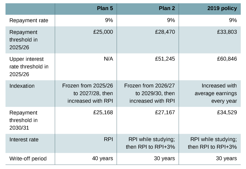
_{Note: 2019 policy thresholds reflect Plan 2 thresholds if 2019 values (£25,725 and £46,305) had been increased in line with average earnings growth between 2019/20 and 2025/26 as per estimates from the Office for Budget Responsibility (OBR)’s Economic and Fiscal Outlook, March 2026. Interest is always applied reflecting OBR forecasts for RPI from 2025/26 onwards.}

Direct grants to universities

Some subjects attract additional direct grant funding where they are particularly high-cost for universities to deliver. We map each subject onto the subject price groups (A to C1.2) they were assigned to in the 2025/26 academic year. We estimate spending on each student each year based on the relevant funding rate per full-time equivalent (FTE) in 2025/26 from Office for Students (2025b, table 5) and assume these rates are fixed over time in CPI real terms.

Income tax and National Insurance contributions

Table B.3 shows the thresholds and rates at which we apply income tax and National Insurance contributions (NICs) in the 2025/26 tax year for our main estimates. We reflect planned cash-terms freezes in personal tax thresholds until April 2031, after which all thresholds are assumed to increase each year in line with forecast CPI inflation. The final column shows the rates and thresholds applied in Chapter 7, to approximately match 2019/20 tax policies with thresholds expressed in 2025/26 prices.

Table B.3. Income tax and National Insurance contributions

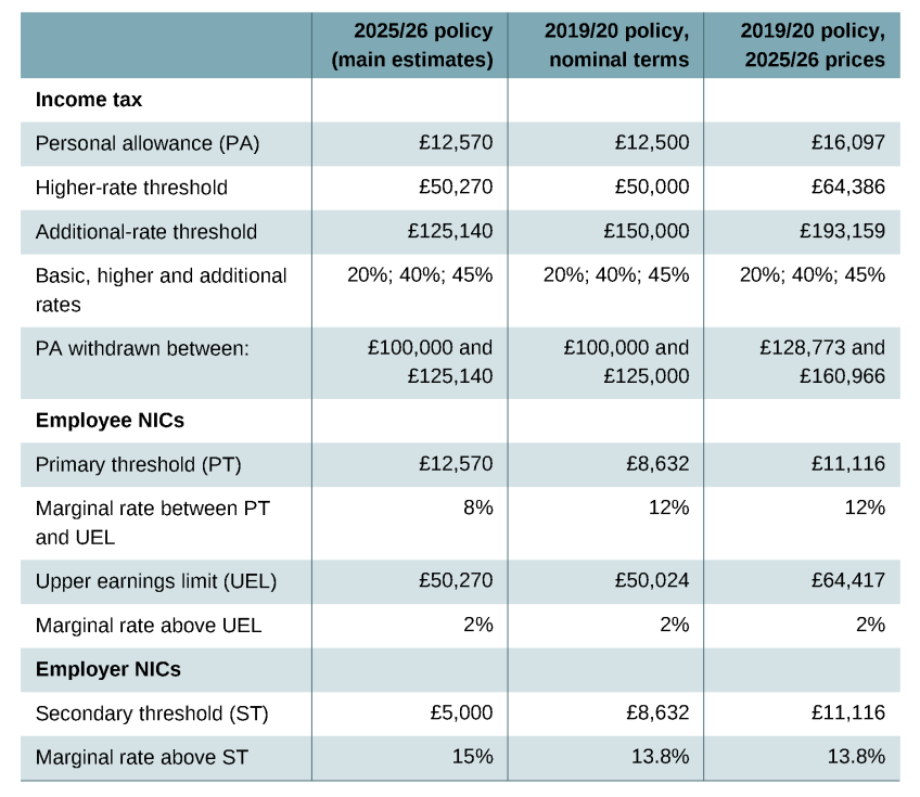
_{Note: Thresholds are annual equivalents and are as applied in the modelling for the 2025/26 tax year. Modelling does not reflect withdrawal of child benefit.}

Modelling changes between this report and Britton et al. (2020)

Both this report and Britton et al. (2020) estimate lifetime returns to undergraduate degrees, focusing on the 2002 GCSE cohort, using the LEO, HESA–HMRC and LFS data, and applying very similar methodologies. However, there are differences in the years of data we use and in the government policy we model, as described in Chapter 7.

Figure 7.1 decomposes the impact of these various changes on our overall average estimated returns, and includes an ‘other’ bar. This captures a range of other factors that will have contributed to changes in the overall returns estimates but which it is difficult to consider separately. Some of these reflect changes to the data, in particular: we now use updated identifiers linking the NPD, HESA and HMRC datasets together, and have improved match rates; we define subjects using the most recent version of the CAH classification, rather than the version that was current as of 2020; we now have and are able to use additional data for tax years 2003/04 and 2004/05 (ages 17 and 18 for the cohort of interest); and we have revised, more accurate inflation figures for the late 2010s, which are used to convert earnings to today’s prices.

Other factors reflect choices we have made to diverge slightly from the methodology used previously, where there was a compelling reason to do so. For instance, we now restrict our sample to those scoring at least the points equivalent of five C grades in their top eight GCSEs, while Britton et al. (2020) required at least five A*–C grades. This less restrictive criterion allows us to retain some more individuals with relatively low prior attainment, which is particularly important now we consider returns for later cohorts as well, given that the expansion of HE participation in recent years has been greater amongst students with lower prior attainment. We also choose a slightly simpler set of variables to control for socio-economic status in our regressions (IDACI (Income Deprivation Affecting Children Index), eligibility for free school meals, and whether a student went to independent school).

The net effect of all of these ‘other’ changes is small but positive for both men and women.

Appendix C. Distribution of age 37 earnings by subject 

For women from the 2002 GCSE cohort, median pre-tax annual earnings at age 37 (among those who had positive earnings in that tax year) ranged from around £30,000 (in today’s prices) for those who studied creative arts, social care, education and performing arts, up to around £40,000 amongst those who studied computing, languages and business. The highest median earnings for women were amongst those who studied medicine (£65,000) and economics (£68,000). 

For men, many of the same subjects as for women had the lowest median earnings at age 37, with median earnings among non-graduate men and those who studied agriculture and creative and performing arts at around £40,000. Median earnings were between £60,000 and £70,000 among male graduates of politics, law, physics, engineering and medical sciences, and were highest among men who studied economics (£90,000) and medicine (£103,000).

As shown in Figure C.1, there was also substantial variation in gross annual earnings among women and among men who had studied the same subjects. This means that there was substantial overlap in the distribution of earnings among those who studied different subjects, even where these had very different median earnings. For instance, the highest-earning quarter of men who studied creative arts earnt more than £60,000 at age 37, more than the lowest half of male earners from all except the highest-earning eight subjects. 

Figure C.1. Distribution of gross earnings at age 37 by subject

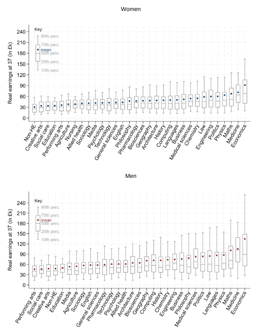
_{Note: Excludes zero earnings. Subjects ordered by mean earnings. Sample selected as discussed in Section 2.1.}

Across both men and women, there was more variation in the earnings of those who studied economics than among medics. For instance, the middle-earning half of male economics graduates with positive earnings earnt between £55,000 and £149,000 at age 37, compared with a narrower range of £67,000 to £139,000 for male medicine graduates. Nursing stands out as having the smallest range in graduate earnings for women: the middle-earning half of women who studied nursing earnt between £27,000 and £50,000, and the 10th percentile of female nursing graduates earnt £16,000, more than the 10th percentile of female physics graduates.

Appendix D. Total returns

Total returns can be thought of as the overall earnings impact of undergraduate degrees, irrespective of to whom these earnings accrue. It differs slightly from gross earnings returns as it includes the effect of undergraduate education on employer National Insurance contributions and takes into account the cost of providing higher education. The average total return per student in discounted present-value terms is around £138,000 for women and around £216,000 for men, with Green Book discounting (Table D.1). 

Table D.1. Average total lifetime returns and share achieving positive returns

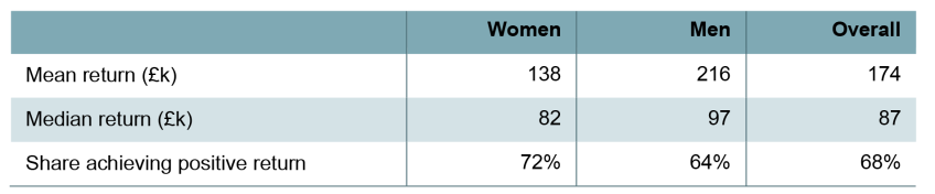
_{Note: All figures are shown in 2025/26 CPI prices and are discounted using Green Book discounting.}

These numbers depend crucially on the discount rate: average (mean) undiscounted total returns are around £497,000 for women and £811,000 for men (Figure D.1). Total returns for both men and women turn positive from age 39 for women and age 42 for men, with Green Book discounting, reflecting the high up-front cost of degrees in terms of both forgone earnings and the cost of providing higher education (tuition fee loans plus teaching grants).

Figure D.1. Mean cumulative total returns to higher education by age

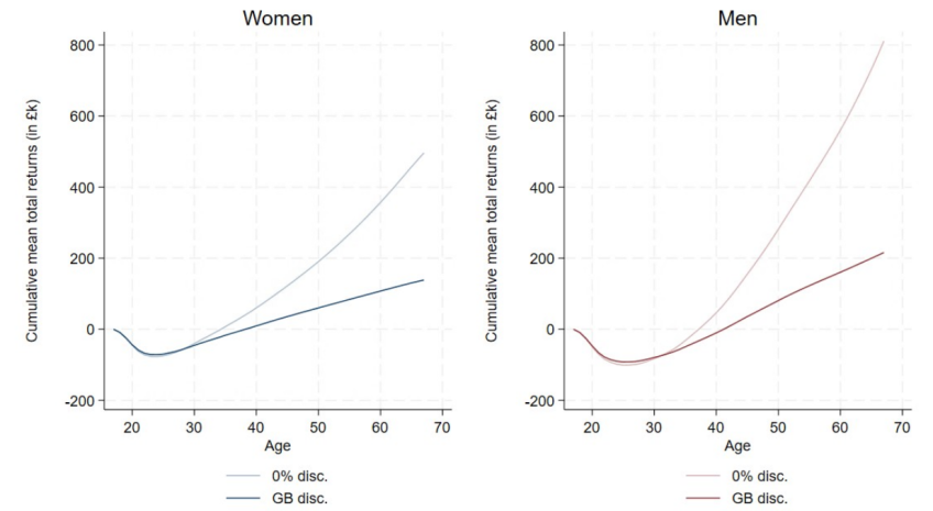
_{Note: All figures are shown in 2025/26 CPI prices and are discounted using either Green Book (GB) discounting, as in our main estimates, or with a 0% real discount rate. Returns at a given age are discounted cumulative returns to that age.} 

Appendix E. Share with positive returns by subject group

Figure E.1. Share with positive net lifetime individual returns to higher education by subject group

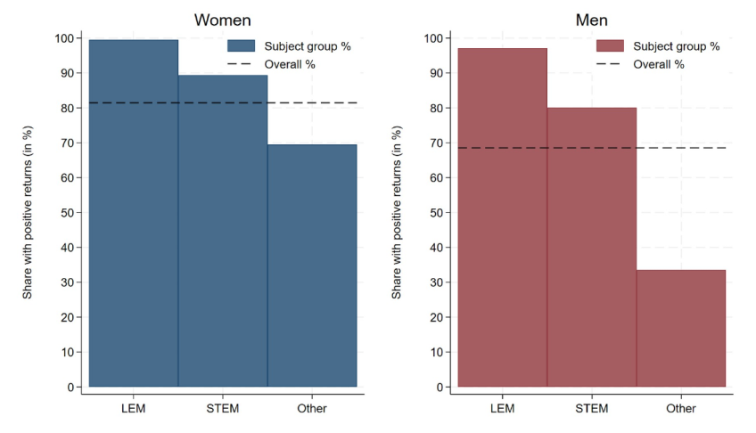
_{Note: Share of individuals for whom we estimate the total lifetime individual return to be positive, with Green Book discounting. Subjects are grouped into STEM subjects (science, technology, engineering and maths), LEM subjects (law, economics and management) and other first undergraduate degrees.}

Figure E.2. Share with positive net exchequer returns to higher education by subject group 

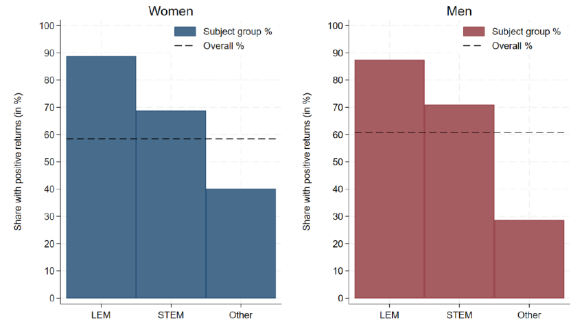
_{Note: See note to Figure E.1. This figure is the equivalent for exchequer returns.}

Appendix F. Lifetime exchequer returns by subject and institution type

Figure F.1. Lifetime exchequer returns to higher education by subject

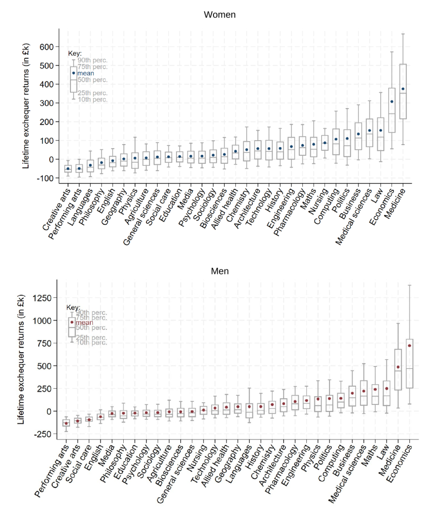
_{Note: All figures are shown in 2025/26 CPI prices and are discounted using Green Book discounting. Subject classification reflects CAH2 and excludes a small number of subjects due to low sample sizes. Subjects are ordered by mean average returns.}

Figure F.2. Lifetime exchequer returns to higher education by institution type

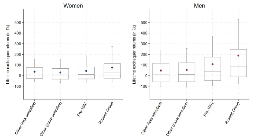
_{Note: Institutions are divided into four groups: Russell Group; old (pre-1992) universities not in the Russell Group; and an ‘other’ category which splits the remaining universities into more and less selective based on the average GCSE point scores of those attending these universities for full-time undergraduate degrees beginning between ages 18 and 20 from the 2002–07 GCSE cohorts.}

Appendix G. Robustness to alternative assumptions

Exchequer returns

Table G.1. Average lifetime exchequer returns, by sex, under different assumptions

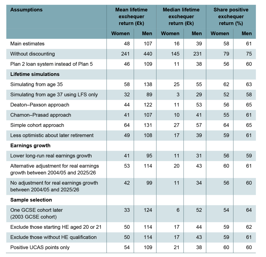
_{Note: Each alternative assumption is applied separately, not in combination. The approach to estimating earning profiles by age from Deaton and Paxson (1994) takes a cohort view, but allows for period effects that are orthogonal to a time trend. The Chamon and Prasad (2010) approach takes a period view and allows for cohort effects that are orthogonal to a time trend.}

Approaches to the age–period–cohort problem

As discussed in Chapter 6, we model various approaches to extracting an age–earnings profile from previous cohorts’ earnings. The fundamental challenge with extracting these profiles is that it is mathematically impossible to separate the effects of age, period and cohort on earnings. For instance, in Figure G.1, we observe that median real earnings among men from the 1978/79 birth cohort were lower at age 43 than at age 42. This will reflect both the fact that the individuals are older (an age effect) and that real earnings across the economy declined in 2022/23 (a period effect), and we cannot disentangle the precise role of each factor. Similarly, earnings at age 42 among men from the 1978/79 birth cohort exceed earnings at 41 among men from the 1979/80 birth cohort. These earnings are from the same tax year (2021/22) but might differ because the two observations are of people at different ages as well as from different cohorts.

Figure G.1. Median real earnings by age for consecutive birth cohorts in the HESA–HMRC data (excluding zeros, 2025/26 prices)

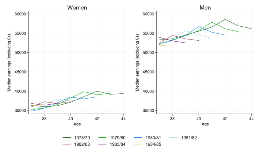
_{Note: HE attendees with positive earnings only. The data cover tax years 2016/17 to 2023/24, which are the years we use in our main results for our simulations of graduates’ earnings up to age 44.}

Estimating the shape of an earnings profile by age therefore requires some assumptions. As discussed in Chapter 6, there are two broad approaches that can be taken to this problem – to take a ‘period view’ or a ‘cohort view’. A simple version of each view assumes there are no other effects, i.e. the ‘simple period view’ assumes there are no cohort effects and the ‘simple cohort view’ assumes there are no period effects. A more complex approach would be to impose some mathematical structure on the other type of effect, rather than assuming it away entirely.

For our main estimates, we apply the ‘simple period view’. This is the simplest and thus most transparent method available, making our results easier to check and replicate for other researchers. It is also the most common method in the literature on the returns to higher education, making our results more comparable to those of other studies, including Britton et al. (2020).

In Chapter 6, we showed that our results are fairly robust to three alternative approaches: a ‘simple cohort view’; a more complex period view following Chamon and Prasad (2010), which assumes any cohort effects are orthogonal to a time trend; and a more complex cohort view following Deaton and Paxson (1994), which assumes any period effects are orthogonal to a time trend. The Deaton–Paxson approach led to higher estimates of individual lifetime returns for men, and the simple cohort view led to higher estimates for both men and women. 

We show more detail on how these alternative assumptions change our lifetime earnings simulations in Figures G.2 and G.3. For women, the simple cohort view is more optimistic than the simple period view for graduates’ earnings up to the early 40s, which produces higher estimates of lifetime returns. For men, higher graduate lifetime earnings under the cohort views are driven by more pessimistic simulations for non-graduate earnings relative to the period views. Equivalent figures are presented in section F of the online appendix to Britton et al. (2020).

Figure G.2. Median actual and simulated gross earnings by age for 2002 GCSE cohort using different simulation methods, for women

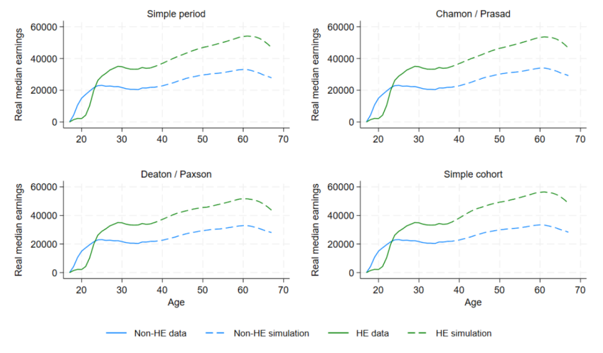
_{Note: ‘HE’ includes those who started a full-time undergraduate degree before the age of 21. Gross annual earnings in 2025/26 CPI prices. Includes zero earnings. Sample selected as discussed in Section 2.1. Data before age 27 exclude self-employment earnings.} 

Figure G.3. Median actual and simulated gross earnings by age for 2002 GCSE cohort using different simulation methods, for men

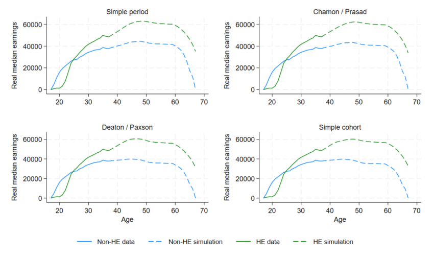
_{Note: ‘HE’ includes those who started a full-time undergraduate degree before the age of 21. Gross annual earnings in 2025/26 CPI prices. Includes zero earnings. Sample selected as discussed in Section 2.1. Data before age 27 exclude self-employment earnings.} 

Appendix H. Comparison of exchequer returns by subject with previous estimates 

Figure H.1. Comparison of average exchequer lifetime returns by subject (2025/26 prices)

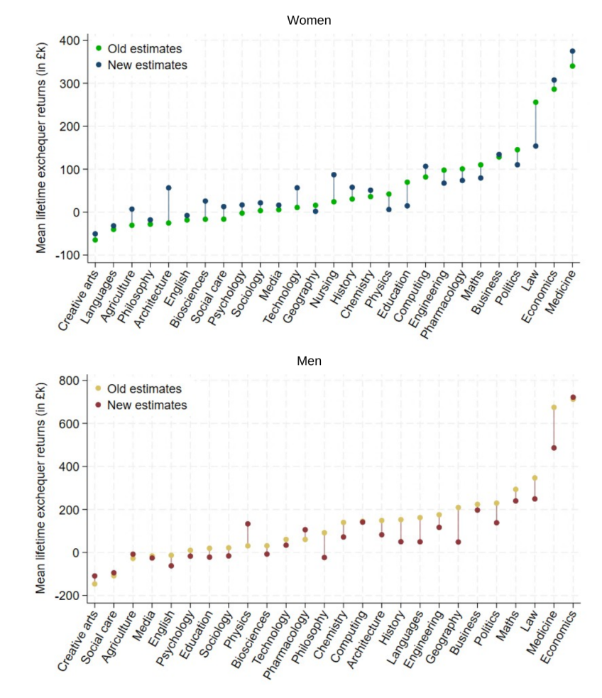
_{Note: ‘Old estimates’ are from Britton et al. (2020), in 2025/26 CPI prices. ‘New estimates’ are the main estimates from this report, and match the averages in Figure F.1. Subjects are ordered by exchequer returns in Britton et al. (2020). Subjects for which HESA’s CAH2 codes have changed substantially between our old and new estimates are not shown. One exception that we do show is ‘Creative arts’, which is compared with ‘Creative and performing arts’ under HESA’s old classification.}

Appendix I. Returns for other prior attainment groups

In Chapter 8, we presented estimates for the lifetime returns to HE among students with ‘low prior attainment’. We defined students as having ‘low prior attainment’ if they had achieved the points equivalent of five C grades but no more than four Bs and four Cs in their top eight GCSEs. This included approximately the bottom 35% of the sample.

Returns for students with lowest prior attainment (bottom fifth)

We also estimate returns for an even smaller subset of the sample: those who achieved at most the points equivalent of eight Cs in their top eight GCSEs. The GCSE passing grade is C, so this is a relatively low bar, corresponding to approximately the bottom 20% of our sample. Amongst this bottom fifth, 45% attended HE.

In Figure I.1, we show cumulative average returns by age for this subgroup, both for individuals and for the exchequer. We estimate average net discounted lifetime returns of £81,000 for women and £34,000 for men in this subgroup, and average exchequer returns of £18,000 for women and £11,000 for men. These are slightly higher for women and slightly lower for men than our estimates based on the bottom 35% of the sample, but overall the estimates are very similar. We estimate negative median exchequer returns for men in the bottom fifth of the sample of –£12,000, compared with –£5,000 when looking at the bottom 35%. 

Figure I.1. Mean cumulative individual and exchequer returns to higher education by age: ‘lowest prior attainment’ group (bottom fifth of our sample)

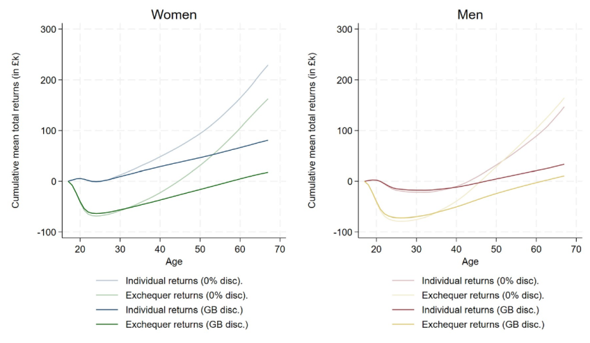
_{Note: See note to Figure 8.4. This figure is equivalent, except that the sample is restricted to students in the bottom fifth of the sample according to their GCSE scores, conditional on meeting the sample criteria.}

In Figure I.2, we show breakdowns of returns for the bottom-attaining fifth of the sample by subject. The order of subjects is mostly consistent with Figure 8.5, though we show fewer subjects here as sample sizes become very small.

Figure I.2. Net lifetime individual returns to higher education by subject: ‘lowest prior attainment’ group (bottom fifth of our sample)

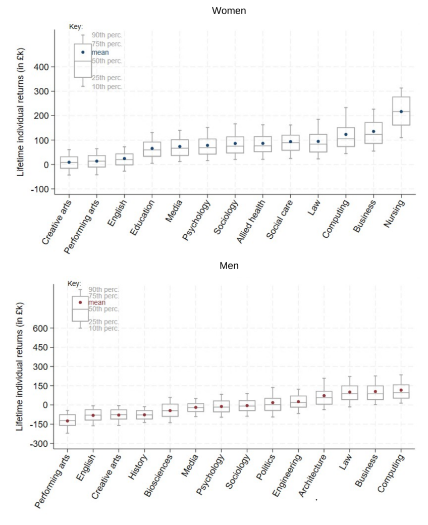
_{Note: See note to Figure 8.5. This figure is equivalent, except that the sample is restricted to students in the bottom fifth of the sample according to their GCSE scores, conditional on meeting the sample criteria.}

Returns for students with medium prior attainment

We also investigate lifetime returns to students with medium levels of prior attainment. We consider the subset of students who achieve above the points equivalent of four Bs and four Cs in their top eight GCSEs, but no more than the points equivalent of four Bs and four As. This approximately corresponds to the students between the 35^th and 70^th percentiles of the main analysis sample in terms of prior attainment. Amongst this subgroup, 83% attended HE. 

Figure I.3 shows mean cumulative average returns to the individual and to the exchequer for this subgroup. These are higher than the cumulative returns we estimate for the low prior attainment subsample for men, and similar for women. We estimate average discounted net lifetime returns to the individual of £75,000 for both men and women, and exchequer returns of £29,000 for women and £67,000 for men. Figure I.4 breaks down individual discounted returns for this subgroup by subject. The patterns remain quite similar to our estimates based on the full sample.

Figure I.3. Mean cumulative individual and exchequer returns to higher education by age: ‘medium prior attainment’ group

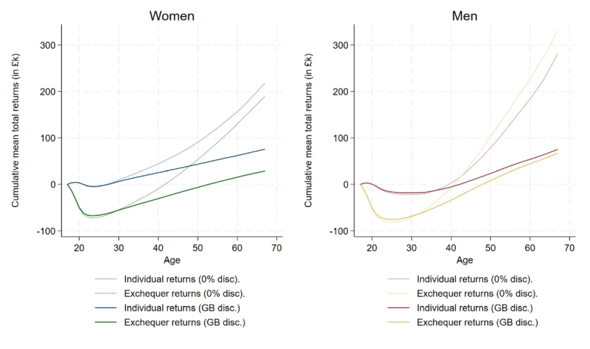
_{Note: See note to Figure 8.4. This figure is equivalent, except that the sample is restricted to students approximately between percentiles 35 and 70 according to their GCSE scores, conditional on meeting the sample criteria.}

Figure I.4. Net lifetime individual returns to higher education by subject: ‘medium prior attainment’ group

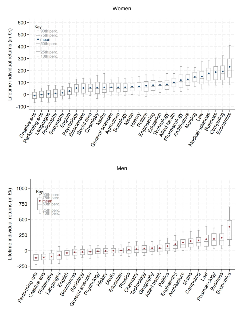
_{Note: See note to Figure 8.5. This figure is equivalent, except that the sample is restricted to students approximately between percentiles 35 and 70 according to their GCSE scores, conditional on meeting the sample criteria.}

One pattern that emerges from our estimates is that while there is a clear relationship between prior attainment and returns for men, this does not seem to be the case for women. For men, we estimate lower returns for the bottom 35% than for students between percentiles 35 and 70. These estimates are in turn lower than our estimates for the full sample, implying higher returns among the top 30% (although we do not estimate lifetime returns at the top of the prior attainment distribution, as there would be too few non-graduates to reasonably simulate earnings up to retirement). For women, this relationship is much less steep. Table I.1 summarises our estimates of lifetime returns for each prior attainment subgroup. 

Table I.1. Average individual and exchequer lifetime returns, and share achieving positive returns, by prior attainment

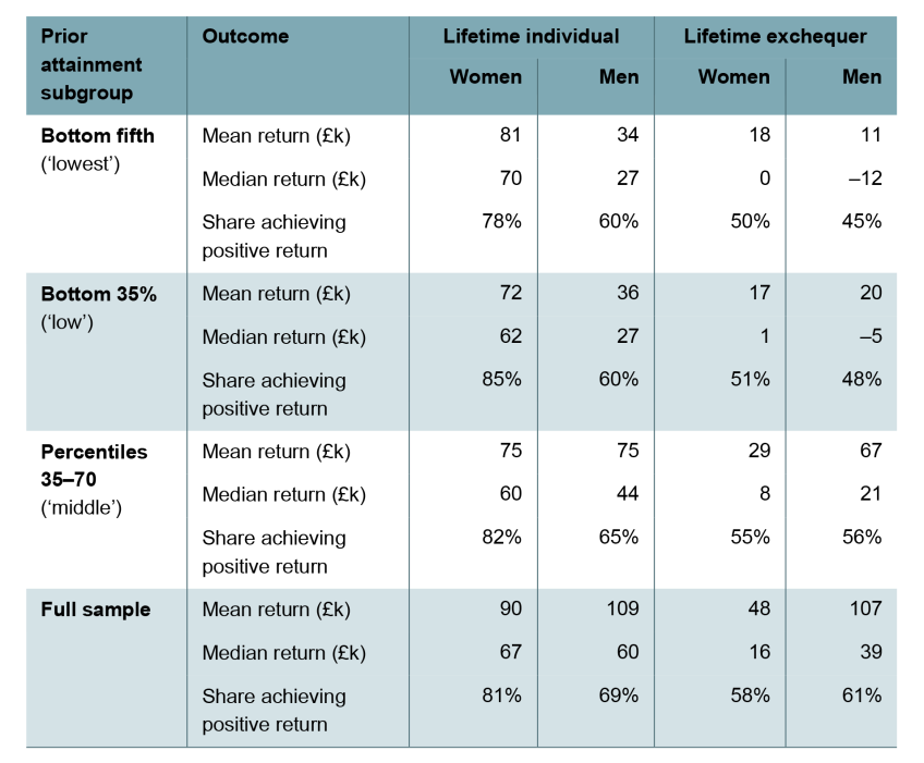
_{Note: All figures are shown in 2025/26 CPI prices and are discounted using Green Book discounting.}

Appendix J. Returns by socio-economic status and ethnicity

This report focuses on how returns vary by subject studied and institution type, rather than on how they vary by background characteristics of the students. In earlier work (Britton, Dearden and Waltmann, 2021) we estimated individual lifetime returns by socio-economic status (SES) at age 16 and by ethnicity. That analysis found that average lifetime returns were positive for men and women from all socio-economic and ethnic groups, although there were substantial differences in average returns between groups. Returns varied little by socio-economic status, with only those who went to independent schools – and particularly men – achieving substantially higher returns, partly reflecting that those from more advantaged socio-economic backgrounds were more likely to study at higher-return institutions. On ethnicity, returns were mostly lower for Black students than for White students, and higher for South Asian students, with subject choice playing a role in explaining these differences.

In this appendix, we provide updated estimates reflecting our updated data and modelling: incorporating data from HMRC records for the 2002 GCSE cohort up to age 37 and simulated data thereafter, following the methodology described in Section 3.1. Any caveats to the analysis described in Britton, Dearden and Waltmann (2021) also apply here.

We begin by showing estimated average net lifetime discounted earnings for graduates and non-graduates by SES group (Figure J.1) and by ethnic group (Figure J.2). These are net of taxes and any net loss (or gain) from student loans, but do not adjust for differences in background characteristics between graduates and non-graduates. These update figures 17 and 18 respectively from Britton et al. (2021).

Figure J.1. Average predicted net lifetime individual earnings by socio-economic status

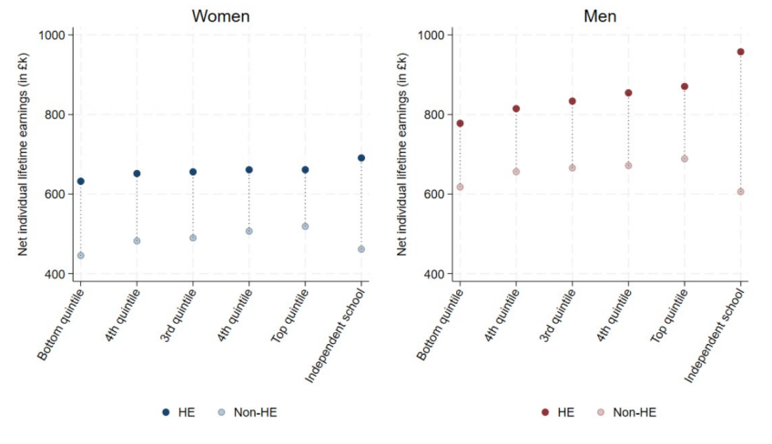
_{Note: Mean predicted lifetime earnings in 2025/26 CPI prices, net of taxes and student loans and discounted using Green Book discounting. HE and non-HE samples selected as described in Section 2.1, and lifetime earnings simulated as described in Section 3.1. Socio-economic status split into quintiles based on IDACI (Income Deprivation Affecting Children Index) score of home address at age 16, and are defined within the full GCSE cohort (rather than within the selected sample). Independent school pupils are shown as a separate category as we rely on a match to School Census records for IDACI scores.} 

Figure J.2. Average predicted net lifetime individual earnings by ethnic group

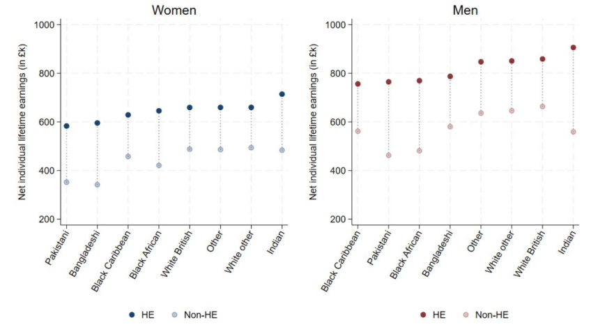
_{Note: Mean predicted lifetime earnings in 2025/26 CPI prices, net of taxes and student loans and discounted using Green Book discounting. HE and non-HE samples selected as described in Section 2.1, and lifetime earnings simulated as described in Section 3.1. Gaps do not correct for differences in background characteristics.}

We then show individual lifetime returns, controlling for background characteristics, for each SES group (Figure J.3) and ethnic group (Figure J.4). These update figures 21 and 23 from Britton et al. (2021).

Figure J.3. Net lifetime individual returns by socio-economic status

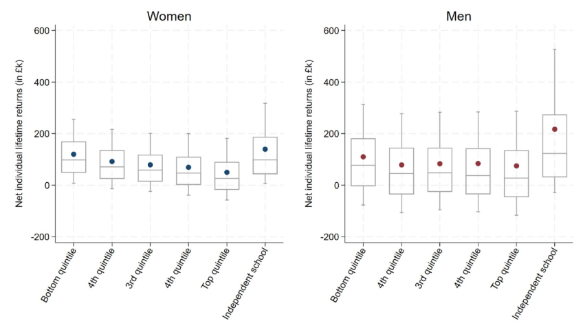
_{Note: Distributions of net lifetime individual returns by socio-economic status. Estimates account for the effect of selection into HE, are net of taxes and student loans, and are discounted using Green Book discounting. See note to Figure J.1 for details on socio-economic status categories.}

Figure J.4. Net lifetime individual returns by ethnic group

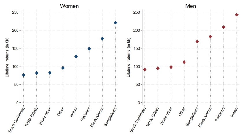
_{Note: Average lifetime returns by ethnic group. Estimates account for the effect of selection into HE, are net of taxes and student loans, and are discounted using Green Book discounting.}

Finally, we show estimates of the share of those attending HE who achieve a positive individual lifetime return, by SES group (Figure J.5) and by ethnic group (Figure J.6). These update figures 22 and 24 from Britton et al. (2021).

Figure J.5. Share with positive lifetime discounted individual return to higher education by socio-economic status

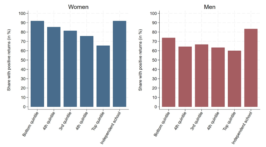
_{Note: Share of individuals for whom we estimate the lifetime individual return to be positive, with Green Book discounting.}

Figure J.6. Share with positive lifetime discounted individual return to higher education by ethnic group

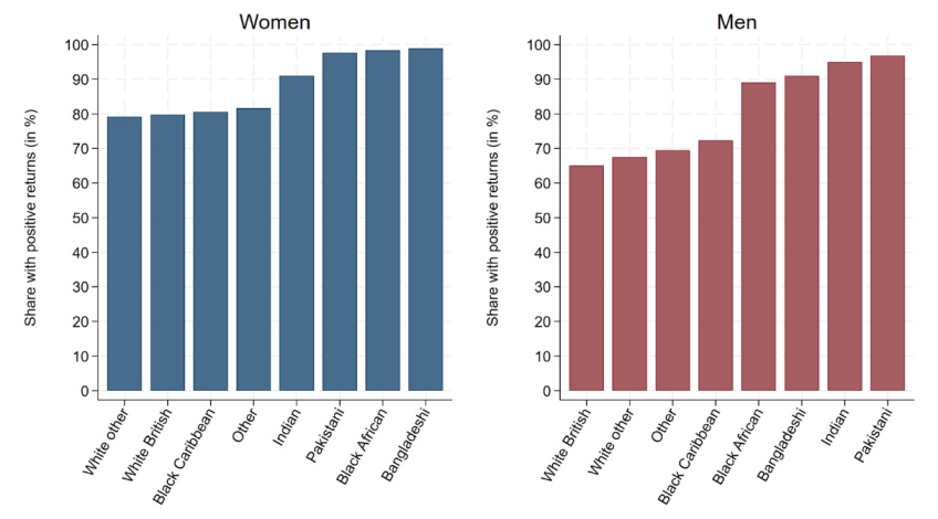
_{Note: Share of individuals for whom we estimate the lifetime individual return to be positive, with Green Book discounting.}

Appendix K. Subject mix over time

Table K.1. Share of HE students (full-time undergraduates starting degrees by age 21) by subject: 2006 and 2022 university entry cohorts

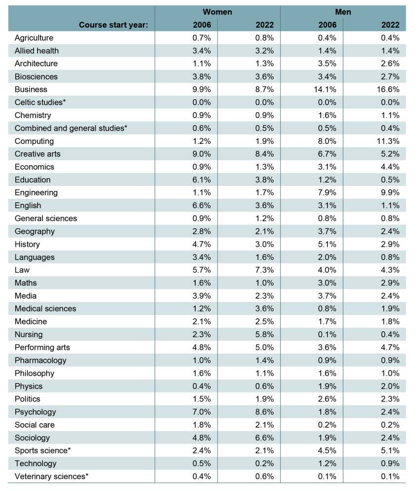
_{Note: Only includes individuals we observe with a KS4 record in LEO. We do not condition on any of our other sample restrictions (minimum GCSE scores, KS5 records or linked HMRC data). Starred subjects are those for which we do not model lifetime returns. Students studying joint degrees are weighted by full-person equivalents.}

Appendix L. Early labour market experiences of later cohorts 

In this appendix, we present median earnings and worklessness rates between ages 24 and 37 for successive GCSE cohorts.54 These can inform us as to whether the earnings and employment of graduates and non-graduates early in their careers have improved or worsened over time, providing suggestive evidence on how returns to university might have changed.

We first present median earnings of graduates and non-graduates, separately by cohort and sex in Figure L.1, for up to 14 consecutive cohorts of students. These are medians in 2025/26 CPI prices excluding those with zero earnings at a given age and are not adjusted for differences in the background characteristics of our HE and non-HE groups. Importantly, unlike when we estimate returns, here we are not restricting our sample to those who have particular minimum GCSE scores, to having a KS5 record or (amongst graduates) to particular subject choices.55 While we still drop people on some particular HE trajectories, this is much closer to comparing earnings amongst all individuals in a cohort who did or did not attend HE – including those for whom attending HE may not have been a realistic option. 

Figure L.1. Median real earnings by age for consecutive GCSE cohorts amongst men and women who did and did not attend higher education (excluding zeros, 2025/26 prices)

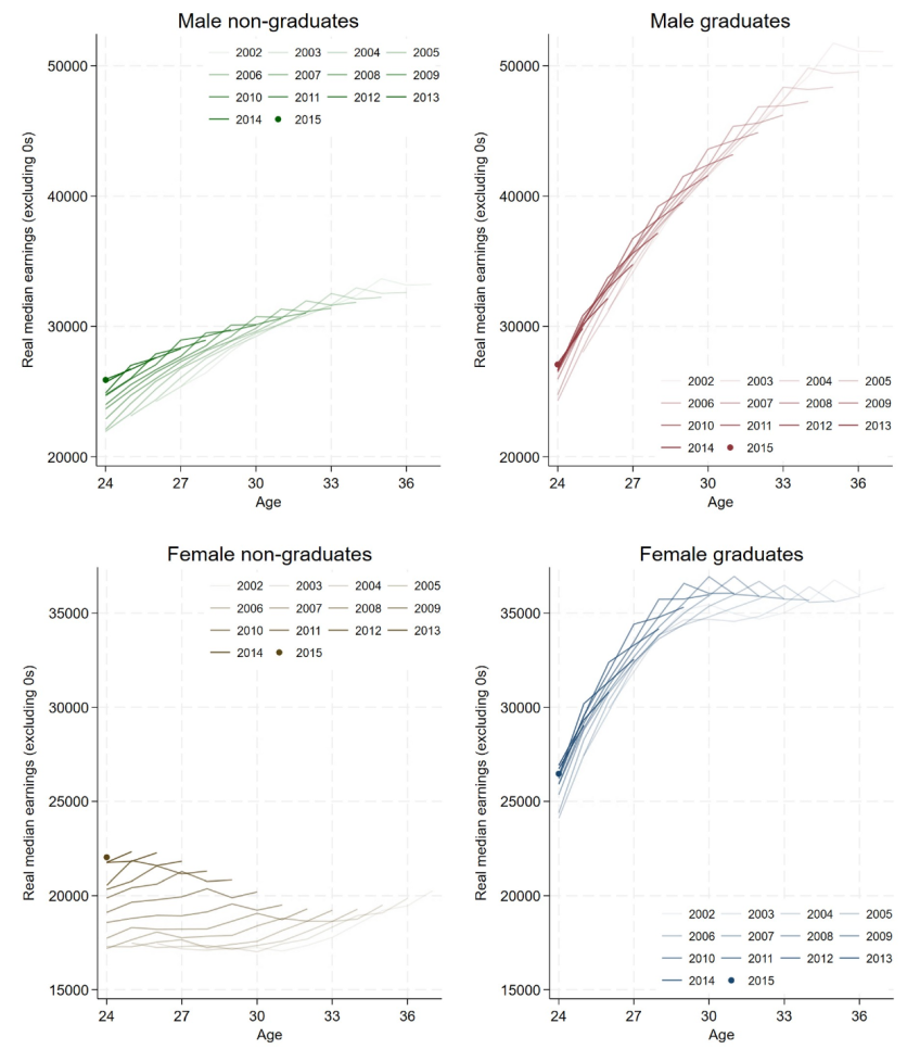
_{Note: Each line relates to a single GCSE cohort: those who took their GCSEs in a given year (from 2002 to 2015). We do not condition on minimum GCSE scores, KS5 records or (for graduates) subject choice. A small number of students for whom we observe a master’s degree, PGCE or PhD but no lower-level degree are excluded. Our HE group contains those starting full-time undergraduate degrees by age 21, and our non-HE group individuals not going to HE at all or beginning degrees after age 24. Students beginning a part-time undergraduate degree or a degree below undergraduate level up to age 21, or any degree between ages 22 and 24 are dropped. We exclude some ages for some of the earlier cohorts because we do not observe self-employment earnings until 2013. Figures are conditional on observing positive earnings at the relevant age.}

Male non-graduates. At age 30, median earnings of male non-graduates were around £30,000 in today’s prices for all the eight cohorts we observe at that age, with small increases for later cohorts consistent with modest real earnings growth over time. The age profiles are reasonably similar across all cohorts, except that period effects mean economy-wide shocks affect different cohorts at different ages. The spike at age 35 and fall at age 36 for the 2002 GCSE cohort can be seen for all other cohorts at earlier ages, corresponding to strong real earnings growth in 2021/22 followed by the ‘cost-of-living crisis’ in 2022/23.

Male graduates. The earnings profiles of male graduates follow the same pattern, although the relationship between median earnings and age is much steeper – reflecting that graduate men tend to see faster earnings growth during their 20s and 30s than non-graduate men. While median earnings are similar to male non-graduates’ earnings at age 24, by age 30 the median male graduate’s earnings are approximately £42,000, roughly 40% higher than the median earnings of male non-graduates of the same cohorts at age 30. 

That said, at earlier ages, there seems to be less cohort-on-cohort earnings growth for male graduates than for non-graduates. Between the 2005 and 2015 GCSE cohorts, earnings at age 24 grew by 18% for non-graduate men (from £22,000 to £25,900 in today’s prices), but by just 11% for graduate men (from approximately £24,300 to £27,100). This may partly reflect that the adult minimum wage has been increasing faster than inflation and increasing as a proportion of economy-wide median earnings since the early 2000s (Francis-Devine, 2026).

Female graduates. For graduate women, the early age–earnings relationship looks similar to that of male graduates. There is a clear positive relationship between age and earnings until around age 30, when earnings amongst graduate women across eight cohorts were around £35,000 in today’s prices. Amongst the latest (2009) GCSE cohort observed at age 30, median earnings were 78% higher than amongst non-graduate women from the same cohort at the same age. However, median earnings amongst graduate women then plateau up to their mid 30s.

Female non-graduates. This picture looks quite different for non-graduate women. They have seen a large increase in median earnings at younger ages over successive cohorts, and more so than non-graduate men, with median earnings at age 24 increasing by 27% between the 2005 and 2015 GCSE cohorts (from £17,300 to £22,000 in today’s prices). As well as any changes in hourly pay, this will reflect any changes in non-graduate women’s labour supply; the medians capture not just changes in hourly earnings but also shifts away from part-time work towards full-time work and changes in the composition of non-graduate women in work.56 Analysis of the LEO data shows there has been a simultaneous decrease in the share of non-graduate women who have zero earnings (see Figure L.2), something not seen for any other group.

Figure L.2. Worklessness share by age for consecutive GCSE cohorts, for men and women who did and did not attend higher education

_{Note: See note to Figure L.1. Although we use the term ‘worklessness’, we model whether or not people have positive (non-zero) earnings in a given tax year rather than their employment status. We are unable to distinguish between the unemployed and those not looking for work. We treat those in self-employment who had zero or negative profits as not being in work. We also treat those who have emigrated or who have died as not being in work, because we cannot distinguish between these states and worklessness in the tax data.}

Figure L.3 shows the median earnings of graduates and non-graduates in real terms when we restrict our sample to consider only those who had a realistic option of attending HE based on their prior attainment (using the same prior attainment threshold as described in Section 3.4). The earnings trajectories of young graduates (and young non-graduates for whom university was a realistic possibility) look strikingly similar across the 14 GCSE cohorts since 2002.

Figure L.3. Median real earnings by age for consecutive GCSE cohorts, amongst only men and women for whom higher education is a realistic option (excluding zeros, 2025/26 prices) 

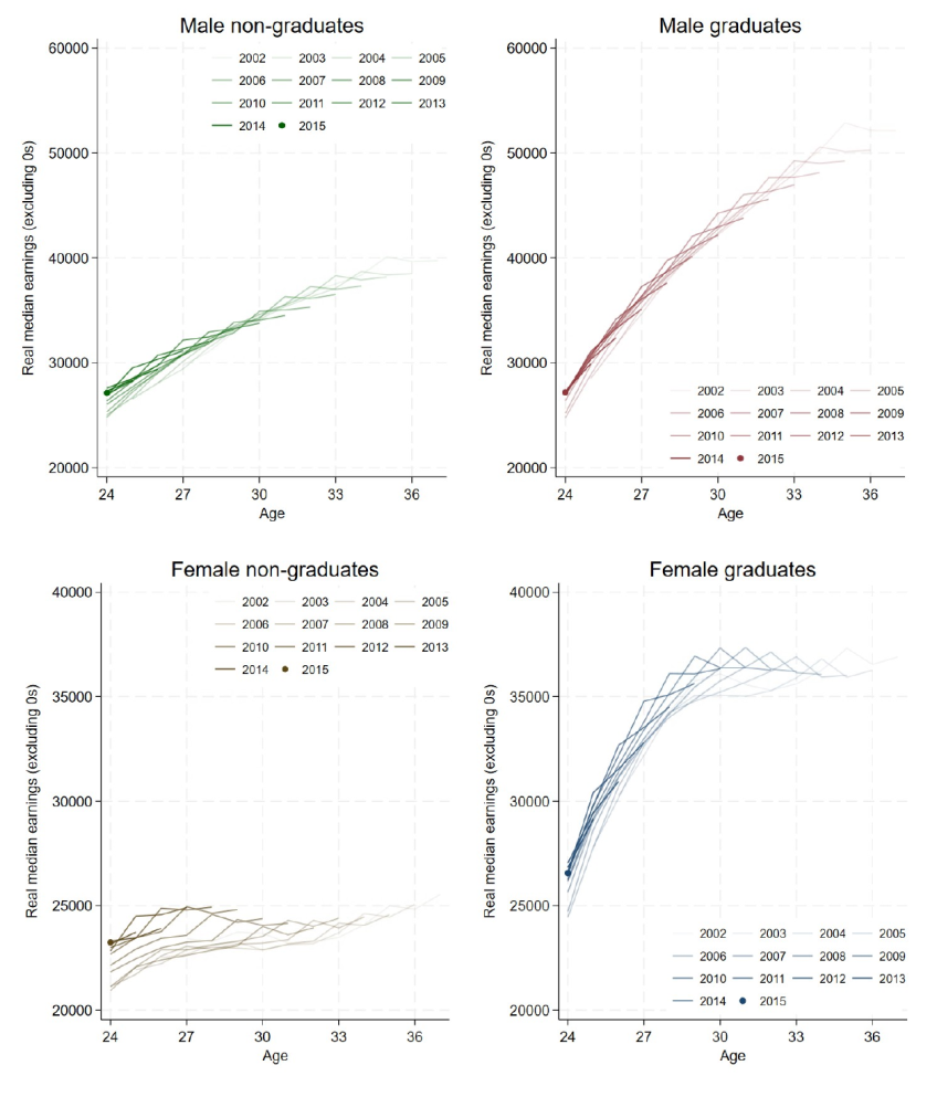
_{Note: See note to Figure L.1. Sample is conditional on minimum GCSE scores and an observed Key Stage 5 record.}

Figure L.4 shows the shares of people with zero earnings in a given tax year for the same groups, i.e. restricting our sample to consider only those who had a realistic option of attending HE based on their prior attainment. The decrease across cohorts in the share of non-graduate women who have zero earnings at younger ages seen on Figure L.2 disappears, suggesting this trend is being driven by non-graduate women who are less comparable to our HE group.

Figure L.4. Worklessness share by age for consecutive GCSE cohorts, amongst only those for whom higher education is a realistic option

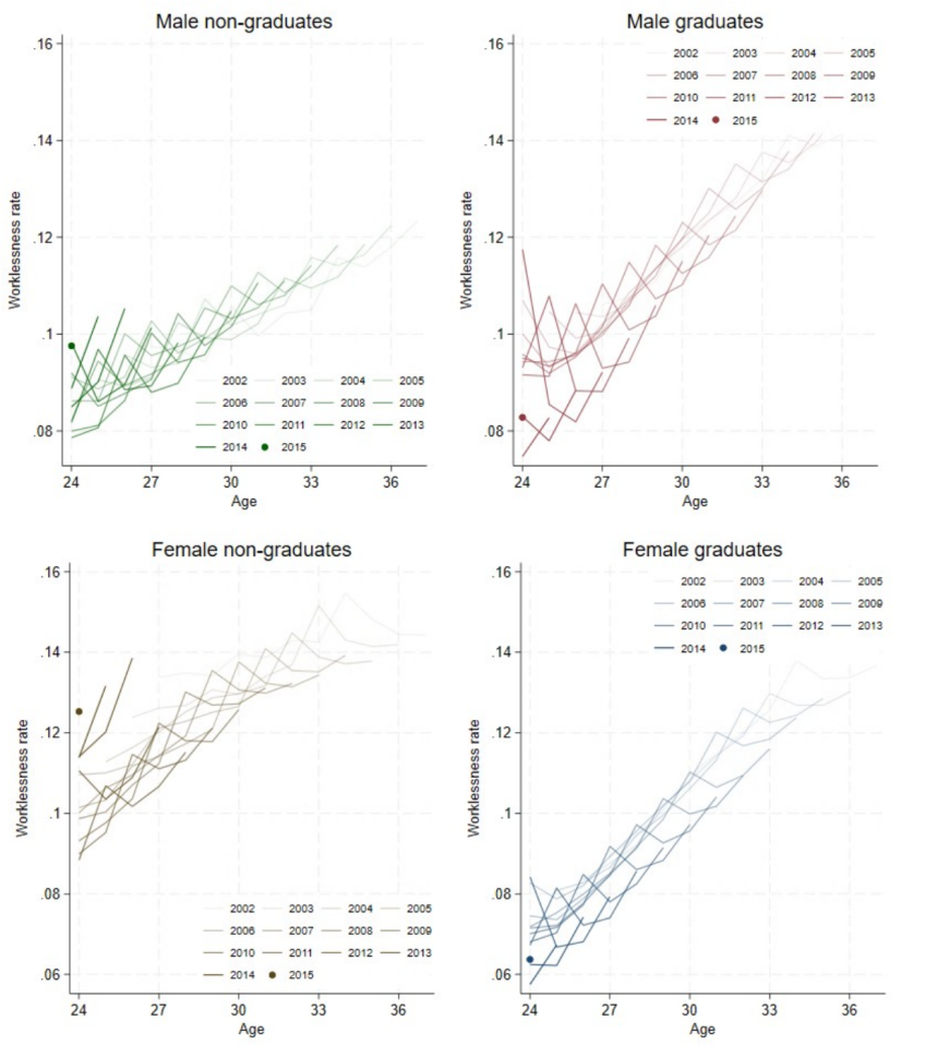
_{Note: See note to Figure L.2. Sample is conditional on minimum GCSE scores and an observed Key Stage 5 record.}

Appendix M. Raw earnings gaps between graduates and non-graduates

In this appendix, we show how raw earnings gaps between graduates and non-graduates have changed over time. To do this, we calculate the difference between average log annual earnings among graduates and non-graduates, and convert this to a percentage difference. We do not account for differences in the background characteristics of those who did and did not attend HE.57 These raw gaps will be larger than the earnings returns to attending HE that we estimate in the text.

We document these gaps in two ways. First, we consider gross earnings gaps across (almost) all individuals in each GCSE cohort, including those who do not have minimum GCSE scores and for whom we do not observe a Key Stage 5 record.58 This is the same approach as is taken in Appendix L. As discussed in Chapter 8, for many individuals in this category, attending HE (at least before age 21) will not have been a realistic option.

These results are shown in Figure M.1. For men, raw earnings gaps between graduates and non-graduates widen with age (each line showing that the gap at a specific age lies above the gaps at earlier ages). In contrast, for women, the gap grows between ages 26 and 30, then shrinks between ages 31 and 37. This is consistent with the plateaus in women’s median earnings around age 30 seen in Figure L.1. The raw earnings gap also appears to decline slightly over successive cohorts. This decline is subtle for men, whereas it is stronger for women, especially among later cohorts. Between the 2005 and 2013 GCSE cohorts, the raw earnings gap for women aged 26 fell from over 80% to under 60%. This is consistent with strong cohort-on-cohort earnings growth among non-graduate women in their 20s, as seen in Figure L.1.

Figure M.1. Raw earnings gaps (in %) at ages 26–37 for successive GCSE cohorts, including those for whom higher education is not a realistic option

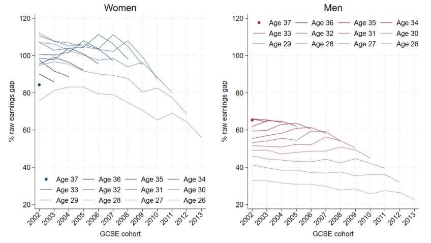
_{Note: Results are based on a calculation of the difference in means of log earnings between individuals who did and did not attend HE. We do not control for background characteristics. Figures are conditional on observing positive earnings at a given age. Earnings at age 26 for the 2002 GCSE cohort exclude self-employment earnings. Sample is not conditional on any minimum school attainment or having a Key Stage 5 record.}

In Figure M.2, we consider the differences in earnings between graduates and non-graduates when we restrict our sample to consider only those who had a realistic option of attending HE based on their prior attainment (using the same prior attainment threshold as described in Section 3.4). The striking finding is that once we focus on this population, raw earnings gaps between graduates and non-graduates at a given age are flat over time (across consecutive cohorts), despite a large increase in HE participation over these cohorts. For neither men nor women do we see any compelling evidence that raw earnings gaps at specific ages have changed substantially between successive cohorts. This is consistent with the earnings trajectories shown in Figures L.3 and L.4

Figure M.2. Raw earnings gaps (in %) at ages 26–37 for successive GCSE cohorts, amongst only those for whom higher education is a realistic option

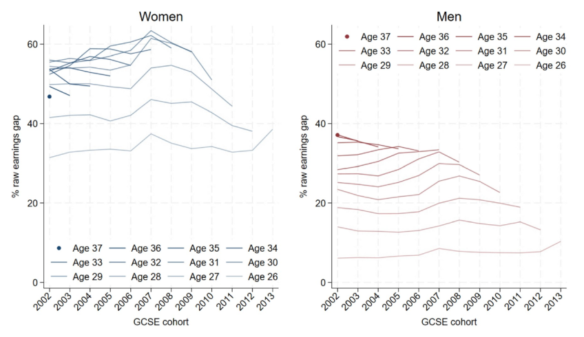
_{Note: Results are based on a calculation of the difference in means of log earnings between individuals who did and did not attend HE. We do not control for background characteristics. Figures are conditional on observing positive earnings at a given age. Earnings at age 26 for 2002 GCSE cohort exclude self-employment earnings. Sample is conditional on minimum GCSE scores and an observed Key Stage 5 record. See Sections 2.1 and 3.4 for details of how we define HE and non-HE groups and which HE trajectories we exclude.}

Appendix N. List of universities by institution type

Institutions are divided into four groups: Russell Group; pre-1992 universities that are not in the Russell Group; and an ‘other’ category which splits the remaining universities into more and less selective based on the average GCSE point scores of those attending these universities for full-time undergraduate degrees beginning between ages 18 and 20 from the 2002–07 GCSE cohorts. A small number (6) of starred providers have been categorised differently from in Britton et al. (2020). Some universities are not listed because they did not exist or had very small sample sizes for these cohorts; for our main estimates, they are grouped with the ‘Other (more selective)’ universities. 

Russell Group

Cardiff University; Imperial College London; King’s College London; London School of Economics; Oxford University; Queen Mary, University of London; Queen’s University Belfast; University College London; University of Birmingham; University of Bristol; University of Cambridge; University of Durham; University of Edinburgh; University of Exeter; University of Glasgow; University of Leeds; University of Liverpool; University of Manchester; University of Newcastle Upon Tyne; University of Nottingham; University of Sheffield; University of Southampton; University of Warwick; University of York

Pre-1992 universities

Aston University; Bangor University; Birkbeck College; Brunel University; City University; Goldsmiths College; Heriot-Watt University, Edinburgh; Keele University; Lancaster University; Loughborough University; Prifysgol Aberystwyth; Royal Holloway; Royal Veterinary College; School of Oriental and African Studies; St George’s Hospital Medical School; Swansea University; University of Aberdeen; University of Bath; University of Bradford; University of Buckingham; University of Dundee; University of East Anglia; University of Essex; University of Hull; University of Kent; University of Leicester; University of London; University of Reading; University of Salford; University of St Andrews; University of Stirling; University of Strathclyde; University of Surrey; University of Sussex; University of Ulster

Other (more selective)

Arts Institute at Bournemouth; Bath Spa University; Bishop Grosseteste University; Bournemouth University; Cardiff Metropolitan University; Central School of Speech and Drama; Conservatoire for Dance and Drama; Courtauld Institute of Art; Glasgow School of Art; Guildhall School of Music and Dance; Heythrop College; Leeds City College; Leeds College of Art and Design; Leeds Metropolitan University; Liverpool Institute for Performing Arts; Liverpool John Moores University; Manchester Metropolitan University; Norwich University College of the Arts; Nottingham Trent University; Oxford Brookes University; Queen Margaret University, Edinburgh; Ravensbourne; Rose Bruford College; Royal Academy of Music; Royal Agricultural College; Royal College of Music; Royal Conservatoire of Scotland; Royal Northern College of Nursing; Sheffield Hallam University; St Mary’s University, Twickenham*; Trinity Laban Conservatoire; University College Falmouth; University of Brighton; University of Chester; University of Chichester; University of Cumbria; University of Glamorgan; University of Gloucestershire; University of Lincoln; University of Northumbria at Newcastle; University of Plymouth; University of Portsmouth; University of St Mark and St John*; University of the Arts London; University of the West of England; University of Wales Trinity Saint David*; University of Winchester; University of Worcester; Writtle College; York St John University College

Other (less selective)

Anglia Ruskin University; Birmingham City University*; Buckinghamshire New University; Canterbury Christ Church University; Coventry University*; De Montfort University; Edge Hill University; Edinburgh Napier University; Glasgow Caledonian University; Glyndwr University; Kingston University; Leeds Trinity University College; Liverpool Hope University; London Metropolitan University; London South Bank University; Middlesex University; Newman University; Robert Gordon University; Roehampton University; Southampton Solent University; Staffordshire University; University Campus Suffolk; University College Birmingham; University for the Creative Arts; University of Abertay Dundee; University of Bedfordshire; University of Bolton; University of Central Lancashire; University of Derby; University of East London; University of Greenwich; University of Hertfordshire; University of Huddersfield*; University of Northampton; University of Sunderland; University of Teesside; University of the West of Scotland; University of West London; University of Westminster; University of Wolverhampton

References

Blundell, R., Green, D. A. and Jin, W., 2022. The U.K. as a technological follower: higher education expansion and the college wage premium. Review of Economic Studies, 89(1), 142–80, https://doi.org/10.1093/restud/rdab034.

Boero, G., Nathwani, T., Naylor, R. and Smith, J., 2025. The college wage premium in the UK: decline and fall? Oxford Economic Papers, 77(1), 1–18, https://doi.org/10.1093/oep/gpae014.

Britton, J., Dearden, L. and Waltmann, B., 2021. The returns to undergraduate degrees by socio-economic group and ethnicity. IFS report, https://ifs.org.uk/publications/returns-undergraduate-degrees-socio-economic-group-and-ethnicity.

Britton, J., Dearden, L., van der Erve, L. and Waltmann, B., 2020. The impact of undergraduate degrees on lifetime earnings. IFS report, https://ifs.org.uk/publications/impact-undergraduate-degrees-lifetime-earnings.

Britton, J. and Gruber, J., 2020. Do income contingent student loans reduce labor supply? Economics of Education Review, 79, 102061, https://doi.org/10.1016/j.econedurev.2020.102061.

Chamon, M. D. and Prasad, E. S., 2010. Why are saving rates of urban households in China rising? American Economic Journal: Macroeconomics, 2(1), 93–130, https://doi.org/10.1257/mac.2.1.93.

Cribb, J. and O’Brien, L., 2024. Recent trends in public sector pay. IFS report, https://ifs.org.uk/publications/recent-trends-public-sector-pay.

Deaton, A. S. and Paxson, C., 1994. Saving, growth, and aging in Taiwan. In D. A. Wise (ed.), Studies in the Economics of Aging, University of Chicago Press.

Department for Education, 2025a. Student loan forecasts for England. https://explore-education-statistics.service.gov.uk/find-statistics/student-loan-forecasts-for-england/2024-25.

Department for Education, 2025b. LEO graduate and postgraduate outcomes. https://explore-education-statistics.service.gov.uk/find-statistics/leo-graduate-and-postgraduate-outcomes/2022-23.

Department for Education, 2026. Participation measures in higher education. https://explore-education-statistics.service.gov.uk/find-statistics/participation-measures-in-higher-education/2023-24.

Department for Work and Pensions, 2025. Third state pension age review: independent report call for evidence. https://www.gov.uk/government/calls-for-evidence/third-state-pension-age-review-independent-report-call-for-evidence/third-state-pension-age-review-independent-report-call-for-evidence.

Francis-Devine, B., 2026. National minimum wage statistics. House of Commons Library research briefing, https://commonslibrary.parliament.uk/research-briefings/cbp-7735/.

HM Treasury, 2026. Green Book supplementary guidance: discounting. https://www.gov.uk/government/publications/green-book-supplementary-guidance-discounting.

Meghir, C. and Phillips, D., 2010. Labour supply and taxes. In J. Mirrlees, S. Adam, T. Besley, R. Blundell, S. Bond, R. Chote, M. Gammie, P. Johnson, G. Myles and J. Poterba (eds), Dimensions of Tax Design: The Mirrlees Review, Oxford University Press. https://ifs.org.uk/books/labour-supply-and-taxes.

Office for Budget Responsibility, 2019. Supplementary forecast information release: long-term economic determinants – March 2019. https://obr.uk/supplementary-forecast-information-release-long-term-economic-determinants-march-2019/.

Office for Budget Responsibility, 2025. Long-term economic determinants – March 2025 Economic and fiscal outlook. Available at https://obr.uk/supplementary-forecast-information-on-long-term-economic-determinants-and-personal-independence-payment-policy-costing/.

Office for Budget Responsibility, 2026a. Supplementary forecast information release: long-term economic determinants – March 2026. https://obr.uk/supplementary-forecast-information-release-long-term-economic-determinants-march-2026/.

Office for Budget Responsibility, 2026b. Economic and fiscal outlook – March 2026. https://obr.uk/efo/economic-and-fiscal-outlook-march-2026/.

Office for National Statistics, 2024. Births by parents’ characteristics. Dataset, https://www.ons.gov.uk/peoplepopulationandcommunity/birthsdeathsandmarriages/livebirths/datasets/birthsbyparentscharacteristics/2021.

Office for National Statistics, 2026a. HOUR01 SA: actual weekly hours worked (seasonally adjusted). https://www.ons.gov.uk/employmentandlabourmarket/peopleinwork/earningsandworkinghours/datasets/actualweeklyhoursworkedseasonallyadjustedhour01sa.

Office for National Statistics, 2026b. EARN01: Average weekly earnings. https://www.ons.gov.uk/employmentandlabourmarket/peopleinwork/earningsandworkinghours/datasets/averageweeklyearningsearn01.

Office for Students, 2025a. Student characteristics data: population data dashboard. https://www.officeforstudents.org.uk/data-and-analysis/student-characteristics-data/population-data-dashboard/.

Office for Students, 2025b. Funding for 2025–26: decisions and allocations. https://www.officeforstudents.org.uk/publications/funding-for-2025-26-decisions-and-allocations/.

Plaister, N., 2022. Why were GCSE grades in independent schools so high during the pandemic? FFT Education Datalab, https://ffteducationdatalab.org.uk/2022/06/why-were-gcse-grades-in-independent-schools-so-high-during-the-pandemic/.

Schulhofer-Wohl, S., 2018. The age-time-cohort problem and the identification of structural parameters in life-cycle models. Quantitative Economics, 9(2), 643–58, https://doi.org/10.3982/QE738.

Stansbury, A., Turner, D. and Balls, E., 2023. Tackling the UK’s regional economic inequality: binding constraints and avenues for policy intervention. Contemporary Social Science, 18(3–4), 318–56, https://doi.org/10.1080/21582041.2023.2250745.

UCAS, 2025. UCAS undergraduate end of cycle data resources 2025. https://www.ucas.com/data-and-analysis/undergraduate-statistics-and-reports/ucas-undergraduate-end-of-cycle-data-resources-2025.

Walker, I. and Zhu, Y., 2013. The impact of university degrees on the lifecycle of earnings: some further analysis. Department for Business, Innovation and Skills (BIS) Research Paper 112, available at https://www.gov.uk/government/publications/university-degrees-impact-on-lifecycle-of-earnings.

Data

Department for Education. HM Revenue and Customs. Department for Work and Pensions. Higher Education Statistics Agency. (2026). Longitudinal Education Outcomes dataset – custom extract provided by Department for Education. https://doi.org/10.57906/pzfv-d195.

Office for National Statistics. Social Survey Division, Northern Ireland Statistics and Research Agency. Central Survey Unit. (2025). Quarterly Labour Force Survey Person — UK, 1997-2020. [data collection]. ONS Secure Research Service. https://doi.org/10.57906/ns1n-5z24.

Acknowledgements

The authors thank the Department for Education for providing access to data and helping to develop this report. They also thank Lorraine Dearden, Laura van der Erve and others for helping to lay the foundations for this work, many colleagues at IFS and elsewhere for helpful discussions and comments, and Judith Payne for outstanding copy-editing. 

The authors gratefully acknowledge funding from the Department for Education (con_28496) and the support of the ESRC Centre for the Microeconomic Analysis of Public Policy (ES/Z504634/1).