IFS fiscal traffic lights: an explainer of indicators and thresholds

1. Introduction

Every government since 1997 has had a set of fiscal rules – usually two or three main ones, almost always including one related to borrowing and one related to debt. The broad aim of these rules is to provide guardrails to ensure that the government of the day does not set the public finances on an unsustainable course.

But simply knowing whether or not these rules are being met and by how much does not provide a comprehensive picture of the health of the public finances. Fiscal sustainability is nuanced and multi-faceted. In this piece, we set out a range of indicators, across different time periods, and use colour-coding to provide a broad summary of fiscal risks and challenges at a glance. Specifically, we set out the indicators, time periods and thresholds we use for the fiscal traffic lights published in Chapter 2 of the IFS Green Budget 2026. This work builds on the fiscal traffic lights proposed in Zaranko (2026).1 

Importantly, there is room for debate, both about the set of indicators and about the thresholds used to monitor the health of the public finances. We have chosen a set of indicators that, in our view, show the key risks and challenges with the public finances in the medium term. Within indicators, we have used historical and international comparisons, and judgement, to choose the thresholds at which levels of concern change.

In Section 2, we summarise the set of indicators we have chosen for the fiscal traffic lights in Chapter 2 of the IFS Green Budget 2026. We then discuss some general principles for our choices of thresholds in Section 3, before discussing each individual indicator and its thresholds in detail in Section 4. In Section 5, we present traffic lights using the same indicators and thresholds for a range of past Office for Budget Responsibility (OBR) forecasts. This exercise helps to illustrate how our fiscal traffic lights might have assessed different moments in recent fiscal history, and shows how much the outlook for the public finances would need to change to produce, for example, a ‘mostly green’ set of fiscal traffic lights. It also provides an assessment of how the broader health of the public finances developed over the last 15 years. This exercise is, of course, done with the perspective of hindsight. Had we produced fiscal traffic lights 5, 10 or 15 years ago, we most likely would have chosen different thresholds.

2. Indicators illustrating the health of the public finances

In the IFS Green Budget 2026, we produce a set of fiscal traffic lights with 11 indicators, covering three themes of short- and medium-term fiscal sustainability. These indicators are summarised in Table 1. The first theme is ‘borrowing and financing’, which covers differences between revenues and expenditure, as well as how much the government has to raise from financial markets. The second is ‘debt and the balance sheet’, which covers the government’s accumulated assets and liabilities, and how they are set to change as a share of national income. The final theme is ‘debt interest risks’, capturing the costs and risks of servicing debt and how they compare with other countries. We discuss each indicator in more detail in Section 3.

Table 1. Indicators included in the 2026 Green Budget fiscal traffic lights

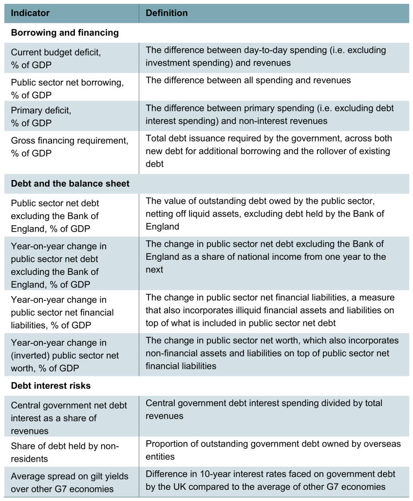
Of course, many of these indicators are closely related to one another. For example, borrowing is typically the most important determinant of year-on-year changes in debt as a share of national income. This means that not every indicator adds completely new information, and it is one reason why the fiscal traffic lights should not be interpreted as a scoring system – five red indicators is not, in any meaningful sense, ‘five times as bad’ as a single red indicator.

For all but two of the indicators, we present their in-year value and their value in the first, third and fifth years of the forecast. For two of them – the share of debt held by non-residents and the average spread on gilt yields over other G7 economies– there is no OBR forecast, such that we use outturn data and show the indicator for the current year only. In all cases, more confidence can be placed on in-year values. Future years are based on forecasts that may not come to pass.

As we have acknowledged above, this set of indicators is not fully comprehensive, and indeed no feasible set of indicators could be. We have chosen a non-exhaustive list of indicators that are useful for assessing the health of the public finances.

Of the indicators we exclude, three are worth highlighting.

First, the expected economic growth rate could be of interest as a standalone indicator; the public finances would be expected to be in better health if, for example, growth was expected to be strong in coming decades. In the set of indicators we use here, we do not include growth, but growth will be reflected in other indicators. Most of our indicators are expressed as a share of national income. This means that if the economy is forecast to be bigger, the same level of borrowing, debt or other fiscal aggregates in cash terms has a lower value as a share of national income and a less concerning colour rating.2 Growth can also affect government revenues and spending, for example through higher tax receipts or lower spending on benefits. A substantial increase in growth would have the effect of driving improvement in many indicators at once.

Second, we do not include longer-term indicators beyond the five years of the OBR forecast. The longer-term view, and issues such as demographic change and rising spending on healthcare will undoubtedly be key to the sustainability of the public finances over the next several decades, while also adding to risks around UK government debt over the next few years. However, while measures of long-term sustainability do exist (e.g. the OBR’s estimate of the primary deficit required to stabilise debt over the long term), they tend to require much more detailed modelling – and a range of assumptions – than medium-term measures. For simplicity, we therefore focus on metrics of sustainability of the public finances over the short and medium term.

Third, we also do not include cyclically adjusted indicators, which explicitly account for the cycle of economic ups and downs. In principle, cyclical adjustment for borrowing measures could provide a better picture of the health of the public finances, by stripping out effects that reflect temporary shocks, and leaving the focus on the more fundamental drivers of borrowing. However, constructing a cyclically adjusted measure requires estimating the gap between actual economic activity – something that is observed noisily and is commonly revised long after the fact – and underlying ‘potential’ economic activity – a concept that can only be estimated, not measured. This estimation is fraught with difficulty, and we take the view that incorporating these cyclically adjusted indicators into the traffic lights would add greater uncertainty rather than clarity.

3. Principles guiding the choice of thresholds

We use a range of six colours in the fiscal traffic lights, as shown by Figure 1. These range from dark green, which represents the lowest level of concern, to red, which represents the highest level of concern.

Figure 1. Colour-coding for the fiscal traffic lights

We judge the degree of concern (and therefore the thresholds that determine the colours) in relation to the medium-term sustainability of the public finances. An indicator is considered more concerning for the sustainability of the public finances if its level or trajectory suggests that the government may face greater difficulty maintaining its fiscal position over time without substantial or disruptive increases in tax or cuts to spending. This may reflect either an increased risk of fiscal stress or crisis, in which the government is forced to make abrupt policy adjustments, or the accumulation of longer-term fiscal pressures that would require significant changes to existing policies even in the absence of a crisis. Some indicators capture vulnerabilities associated with the current fiscal position, such as high levels of debt or debt servicing costs, which can reduce the government’s ability to deal with future adverse shocks and changes in financial market conditions. Others capture risks arising from the projected trajectory of the public finances, such as persistently rising debt, which may increase the scale of future adjustments needed to maintain sustainability. Given this, the ‘least concerning’ level on a given indictor does not imply that the government faces no fiscal constraints from this indicator, but it does mean that the government’s performance on this metric is not likely to generate a significant increase in fiscal risks.

There is no single right or wrong answer as to where the thresholds between colours should lie. Take the current budget deficit as an example: a government running a deficit of 0.5% of national income (which we classify as yellow) is – all else equal – clearly in a less concerning fiscal position than one running a deficit of 2.5% of national income (orange in our classification). The distinction is much less clear, for example, between deficits of 0.9% (yellow) and 1.1% (amber) of national income. But for the fiscal traffic lights to function, thresholds need to be set at some level. The benefit of this approach, however, is that there are five thresholds rather than a single (pass–fail) threshold, which means each threshold is less important.

History can be a useful guide to pick thresholds. For example, we might compare debt this year to debt each year of the past 30 years. If it was higher this year than in 25 of those years (i.e. it was the fifth highest, or higher), we might colour the indicator red, as it would be among the worst outcomes. By the same logic, we might colour it orange if it was higher than in only 20 of those years.

But this historical approach is still sensitive to judgements. For one, averaging over different timeframes will produce very different thresholds, so choosing a timeframe will again require some judgement.3 

An exclusively historical approach also limits the classification of indicators to what has happened in the past, which is not representative of all possibilities. This becomes very clear when we consider what thresholds might have been thought appropriate, had we done this exercise in the past. In 1998, the New Labour government defined a ‘prudent’ level of debt (targeted by its sustainable investment rule, one of the two original fiscal rules) as 40% over the economic cycle.

As the IFS Green Budget 2007 pointed out, this seemed clearly anchored at the level of debt at the time, which was just under 40%.4 This highlights that perceptions of a sustainable fiscal situation are often shaped by the fiscal situation that has been sustained in the recent past. This is understandable, and reasonable up to a point – the fact that the UK is still able to borrow in an orderly fashion from markets does tell us something about the sustainability of its public finances.

More pragmatically, in order for the traffic lights to be a useful communication device, they need to vary across plausible scenarios. So even if a time-traveller from the late 1990s may well find every level of debt that the UK might conceivably have in the next 10 years very concerning (and even if some present-day commentators may agree), traffic lights that are uniformly red are simply not useful outside of a fiscal crisis – instead, in normal times, they should be seen as indicators of the vulnerability to a crisis.

Instead of, or in addition to, using the UK’s own history as comparator, we might consider other countries’ fiscal situation. This can often lead to starkly different assessments. Take public sector net debt, which in 2025–26 stood at 89% of national income – the highest level in the UK for over 50 years.5 This could suggest that the level of debt is currently very concerning. But the UK’s national debt level is below the median of G7 countries, with France, Italy, Japan and the United States all having substantially higher levels. Relying solely on historical comparisons would strip away our ability to distinguish between the UK’s current situation and one where, for example, the UK’s debt-to-GDP ratio was the same as France’s, at around 120%.

The thresholds we have chosen are informed by historical and international data, but also include some judgements. Of course, reasonable people can take different views about the level of concern that a particular indicator warrants. But in the course of operationalising this framework and picking thresholds, we have adhered to a few principles. First, we have used round numbers for each threshold. Second, we have made the distribution of thresholds symmetric. For example, in the case of year-on-year changes in public sector net financial liabilities as a share of national income, the threshold between yellow and amber – the middle of the traffic lights – is zero. The thresholds between light green and yellow and between amber and orange are −1% and 1% of national income, respectively. We have also made the more extreme categories – for example, light green and orange – wider than the less extreme categories (yellow and amber). This enables the traffic lights to adjust more to smaller movements in indicators in less extreme situations (neither particularly good or particularly concerning), while preventing the overall range covered by the whole spectrum of traffic lights from being too narrow.

4. Indicators and thresholds in detail

4.1 Borrowing and financing

4.1.1 Current budget deficit

The current budget deficit is the difference between day-to-day spending and revenues. Achieving a current budget surplus has been one of the government’s primary fiscal rules for 21 of the last 29 years and is included in the current set of fiscal rules. There are good reasons for using this as a rule: it is a reasonable expectation for sustainability that, in normal times, the government is able to cover day-to-day spending solely through revenues. Borrowing for investment is not included in the current budget balance, as the optimal constraints on borrowing for investment might be different: well-targeted investment might boost growth and so alleviate future fiscal challenges. It might therefore be reasonable to think that some costs of investment can be shared with future generations by funding it through borrowing, though it is important that this is not done in an unconstrained manner.6 

Figure 2 shows the thresholds we use for the current budget deficit, centred on a deficit of 1% of national income. The current budget deficit was larger than 1% in four in five years since 2000, making this seem a relatively ambitious threshold. But large current budget deficits were less common across the entire post-war period: it was larger than 1% less than half the time over this longer timeframe.

Figure 2. Thresholds for the current budget deficit

Source: Authors’ calculations.

The thresholds in Figure 2 imply that meeting the government’s current fiscal rule of not borrowing for day-to-day spending in the third forecast year – in other words, running a current budget surplus – would be classified as light green in that year. A current budget deficit of any level would be cause for greater concern.

4.1.2 Public sector net borrowing

Public sector net borrowing (PSNB), also known as the deficit, is the difference between all spending, including on investment, and revenues, measured as a share of national income.

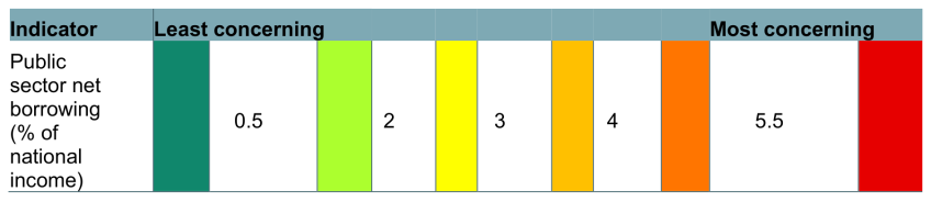
Figure 3 shows our PSNB thresholds, centred on a deficit of 3% of national income. Because PSNB is the sum of the current budget deficit and public sector net investment, a 3% value is compatible with the central value for the current budget deficit we have picked (1% of national income) and the roughly 2% of national income that net investment has averaged over the last 50 years. Countries in the European Union have also used it as a rule-of-thumb upper limit of a sustainable deficit since the introduction of the European Union’s fiscal rules in 1992.

Figure 3. Thresholds for public sector net borrowing

Source: Authors’ calculations.

Since the 1960s, deficits between 0.5% and 2% of national income (light green) have typically been associated with debt falling as a share of GDP. Overall surpluses have been rare – occurring on only five occasions in that same period – so it is reasonable to include a small deficit of under 0.5% of national income in the least concerning category (dark green) category. However, the government has only run a deficit over 5.5% of national income (red) in the post-war period in the immediate aftermath of crises: the 1970s inflation crisis, the 1992 Exchange Rate Mechanism shock, the 2007–08 financial crisis and the COVID-19 pandemic. Anything at or above this level would therefore be very concerning.

4.1.3 Primary deficit

The primary deficit is the difference between spending excluding debt interest and non-interest revenues. When the rate of interest on government debt exceeds the growth rate of the economy, a primary surplus is required for debt to fall as a share of national income. The primary deficit can be seen as a metric of government ‘effort’ to consolidate the public finances, as it accounts for spending other than on servicing debt, which is largely out of the immediate control of any individual government.

Figure 4 shows the thresholds we have chosen for the primary deficit. A deficit of that size or smaller has been achieved six times since the turn of the century. The UK has not run a primary surplus (light green), however, since 2001–02. And while it commonly ran very large primary surpluses that would have been in the dark green category in the 1950s and 1960s, this has only been the case four times since the 1990s.

Figure 4. Thresholds for the primary deficit

Source: Authors’ calculations.

Historically, the debt-stabilising primary deficit – the level of the primary deficit required to keep debt from rising as a share of national income – has been above zero more often than it has been below zero; see Box 4.1 in the OBR’s Economic and fiscal outlook – November 2020. This means that it has often been possible to stabilise, though not meaningfully reduce, debt levels while running a small primary deficit. In line with this, we classify a primary deficit of up to 1% in the yellow category. A primary deficit over 3.5% has happened several times this century, but it has tended to have very bad consequences for levels of debt – the primary deficit was above this level for six years after the Great Recession, in which period debt doubled as a share of national income.

4.1.4 Gross financing requirement

The gross financing requirement measures all cash that the government must borrow from the markets in a given year as a share of national income. This includes both new amounts borrowed and the total value of pre-existing debt that matures in that year and needs to be re-financed through additional borrowing. All else equal, higher borrowing means higher gross financing; but a shorter maturity of debt also pushes up gross financing, as bonds need to be repaid more often. This metric captures exposure to changes in market conditions; the more debt that needs to be issued or rolled over, the more exposed the government is to having to do so at a new and potentially higher interest rate.

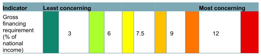
Figure 5 shows the thresholds for the gross financing requirement. We have picked 7.5% of national income as the central point of outcomes – it is close to the average level this century, and roughly in the middle of the extremes that we might consider least and most concerning. The average maturity of UK debt – that is, the average amount of time until debt has to be repaid in full – is nearly 13.5 years.7 At current maturities, the most concerning levels of gross financing would come about with high levels of debt maturing in each year, and high levels of borrowing, and would leave the government very exposed to changes in market conditions. Given the current level of debt, reaching the least concerning end of the spectrum is near impossible: the government is likely to need at least 7% of national income just to redeem existing debt, before any new borrowing in a given year; it is likely to take at least two of lower levels of debt, lower borrowing or longer debt maturities to get the gross financing requirement to a much less concerning level. But it is achievable, particularly if debt is lower: the government reached levels below 3% of GDP in the early 2000s, when debt was lower.

Figure 5. Thresholds for gross financing requirement

Source: Authors’ calculations.

The average maturity of UK debt is lower than in the past, as the government has been issuing a larger share of shorter-dated debt, partly to match changes in demand from investors; see Chapter 2 in the OBR’s Fiscal risks and sustainability – July 2025. Average maturity has fallen by three years in the last decade and, given current government plans to issue less very long-dated debt, falling average maturity seems likely to be the trend going forward, which will push up the gross financing requirement.

The OBR’s forecast of financing requirement over the next five years ranges from 8% to 11% of national income, which would put the traffic light in amber to orange. This is high by historical UK standards. Nevertheless, it remains low compared with other G7 countries. This is because of the UK’s long average maturity of debt relative to other countries. The UK’s debt had an average maturity of 13.5 years in 2024, compared to 8.1 years for France and 5.8 years for the United States. Our judgement is therefore that current levels are not at the highest levels of concern, despite relatively high borrowing, as it would be possible for further shortening in maturities to expose us to meaningfully more risk.

4.2 Debt and the balance sheet

4.2.1 Public sector net debt excluding the Bank of England

Public sector net debt (PSND) is the value of outstanding debt, netted off against liquid assets in the public sector. PSND excluding the Bank of England is also sometimes known as underlying debt, because it excludes the direct effects of monetary policy interventions by the Bank of England, which are outside the government’s control. We therefore use PSND excluding Bank of England in our version of the fiscal traffic lights. For the indicator, we measure this as a share of national income.

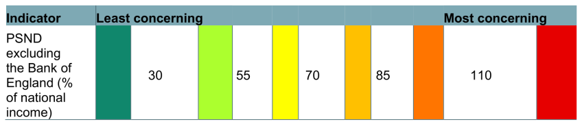
Figure 6 shows our chosen thresholds for PSND. The stock of debt is a key indicator of a country’s fiscal situation and one of the drivers of interest costs. Our choice for the central point is 70% of national income, which means all years since 2010–11 are categorised as amber or worse.

Figure 6. Thresholds for public sector net debt excluding the Bank of England

Source: Authors’ calculations.

PSND excluding the Bank of England was 89% of national income in 2025–26, placing it in the orange category. While this is the highest it has been in over 50 years, it is still lower than that of some comparator economies – for example, France and Italy have government debt of around 120% and 140% of GDP, respectively, both of which we would classify as red. It is therefore reasonable to conclude that the UK’s debt situation is concerning by historical standards, but that it could be more concerning still. As discussed in Section 3, perceptions of a sustainable fiscal situation are often shaped by the fiscal situation that has been sustained in the recent past, and so these thresholds might have looked very different if designed by an observer in the early 2000s. Nevertheless, the fact that the UK is still able to borrow in an orderly fashion from the markets despite much higher debt levels than in the 1990s does tell us something about the sustainability of its public finances.

4.2.2 Year-on-year change in public sector net debt excluding the Bank of England

This is the year-on-year change in PSND excluding the Bank of England, as a share of national income. Every government since 2010 has aimed to get some measure of debt falling relative to national income, and a falling debt-to-GDP ratio, all else equal, would improve the state of the public finances.

Both levels and changes in debt as a share of national income are important indicators of fiscal sustainability. Even if the stock of debt were low, it could be concerning if it was rising quickly; and likewise, even if debt were coming down quickly, it could still be concerning if its level was high.

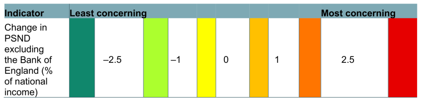
Figure 7 shows the thresholds we have chosen for the year-on-year change in PSND excluding the Bank of England. This is centred on zero, so that debt would be stable as a share of national income, with a fall or increase of under 1 percentage point being yellow or amber, respectively.

Figure 7. Thresholds for the year-on-year change in public sector net debt excluding the Bank of England

Source: Authors’ calculations.

The two largest falls since the turn of the century were a 3.7 percentage point fall in 2017–18 and a 4.2 percentage point fall in 2021–22, both of which would be in dark green. However, the two biggest crises since the turn of the century – the financial crisis and its aftermath (from 2008–09 to 2011–12) and the COVID-19 pandemic (in 2020–21) – would have both been marked as red.

Consistent year-on-year falls in debt would over time reduce the level of debt as a share of national income, although it would be slow. It would take eight years of debt falling by 2.5% of national income (dark green) for the level of debt to fall below 70% of GDP and shift away from being a clear cause for concern (yellow).

4.2.3 Year-on-year change in public sector net financial liabilities

This is the change in the ratio between PSNFL and national income from year to year. PSNFL is a broader measure than PSND excluding the Bank of England; it includes not only liquid liabilities and assets such as outstanding debt and cash held by the government, but also illiquid financial liabilities and assets, such as funded pensions and equity stakes in companies. This means that PSNFL can move in different directions to PSND excluding the Bank of England if there is a substantial change to the value of the government’s net financial assets or if the government issues significant debt to buy financial assets such as equity stakes in companies. One of the government’s fiscal rules mandates that PSNFL should be falling as a share of GDP by the third year of the forecast period.

Figure 8 shows the thresholds we have chosen for the year-on-year change in PSNFL. This is centred on zero, much like the fall in debt as a share of national income, and uses the same thresholds. Different balance sheet metrics measure subtly different things, and the combination can give a more complete picture of the government’s fiscal vulnerabilities than a single measure can. But fundamentally, the same principles that apply to changes in the level of debt – that there is cause for concern if it is rising, and so the traffic lights should be symmetrical around a stable level of debt – also apply to other balance sheet measures.

Figure 8. Thresholds for the year-on-year change in public sector net financial liabilities

Source: Authors’ calculations.

4.2.4 Year-on-year change in (inverted) public sector net worth

This is the change in the ratio between inverted public sector net worth (PSNW) and national income from year to year. Net worth is the broadest measure of the public sector’s balance sheet available for the UK, and includes all the assets and liabilities in PSNFL, as well as non-financial assets and liabilities – for example, the value of land and buildings owned by the government and the liabilities of unfunded public sector pension schemes. Inverting PSNW facilitates comparison with PSNFL and PSND, for which a positive number represents a liability rather than an asset.

Figure 9 shows the thresholds we have chosen for the year-on-year change in PSNW. This is centred on zero, much like the fall in debt as a share of national income, and uses the same thresholds, again due to the same principles.

Figure 9. Thresholds for the year-on-year change in inverted public sector net worth

Source: Authors’ calculations.

Including PSNW allows us to highlight further effects of fiscal policy decisions on different measures of debt and the government’s balance sheet. For example, if the government decided to nationalise a company whose assets are mostly non-financial, such as Thames Water, PSNW would worsen by much less than PSNFL.

4.3 Debt interest risks

4.3.1 Debt interest spending as a share of revenues

Our first indicator in this theme is the proportion of revenue raised in a given year that is spent on servicing debt. The measure of debt interest is net of the effect of quantitative easing/tightening on the government’s accounts, to again separate out the direct effects of monetary policy decisions from our measures of fiscal sustainability.

Figure 10 shows the thresholds we have chosen for debt interest as a share of revenues, with 6% of revenues as the centre of the distribution – the average level over the century so far.

Figure 10. Thresholds for debt interest spending as a share of revenues

Source: Authors’ calculations.

Debt interest as a share of revenues captures the combined effect of the debt stock and the effective interest rate faced by the government, so that higher debt, higher interest rates or both move the indicator further towards red. Debt interest costs in recent years and in the OBR’s March 2026 forecast are high by historical standards, and would be classified mostly as red.

4.3.2 Share of debt held by non-residents

This is the Debt Management Office’s reported share of all outstanding PSND that is held overseas. Overseas investors are often more price-sensitive than domestic buyers, who are either the central bank or might require government debt for regulatory purposes (see Annex 3.A of the OECD’s Global Debt Report 2026). A higher proportion of debt held abroad, then, is likely to leave the government more exposed to sudden changes in global market conditions.8 

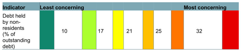
Figure 11 shows the thresholds we have chosen for the share of debt held by non-residents. Levels of foreign holdings vary a lot across the world. For example, Japan has a very low level of foreign holdings (under 10%). Around a quarter of US debt is held abroad, a similar proportion to the Euro Area. The UK, in contrast, has around a third of its debt in the portfolios of foreign investors, marking it out as significantly higher than comparator economies and higher than the OECD average of 28%. In a May 2026 blog ‘The investor base for sovereign debt: why diversification matters’, the OECD identified risks of a rising proportion of developed economies’ debt held overseas – it was 21% in 2007 and 25% in 2022 – and we use those historical values as the centre of the distribution for our indicator.

Figure 11. Thresholds for the share of debt held by non-residents

Source: Authors’ calculations.

4.3.3 Average spread on gilt yields over other G7 economies

This is the difference between the yield – essentially the interest rate – on 10-year UK government bonds (gilts) and the (unweighted) average yield of all other G7 countries (Canada, France, Germany, Italy, Japan and the United States). Market participants generally see 10-year bonds as the benchmark for government debt interest costs, with higher yields often reflecting a higher risk, for which market participants need to be compensated with higher returns.

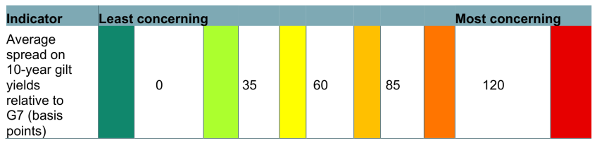
Interest rates on government bonds matter because they affect how much the government has to pay to service a given level of debt. But they are not exclusively driven country-specific factors; for example, there has been a rise in interest rates on government bonds worldwide since the beginning of 2026.9 By focusing on the spread between the UK and other countries, we isolate those global factors that affect interest rates and focus instead on the UK’s risk relative to peer economies. Figure 12 shows the thresholds we have chosen for the spread between the UK’s 10-year gilts and bonds issued by other governments. We have used 60 basis points as the centre of the traffic lights, which is around the average spread since the early 1990s.

Figure 12. Thresholds for the average spread on gilt yields over other G7 economies

Source: Authors’ calculations.

The most desirable situation would be for the UK’s gilts to be trading at a lower yield than the average of its peer economies, which would mean a negative spread – which we have classified as dark green, or least concerning. This has happened only sporadically; mid-2020 was the last time the UK’s gilts traded at a lower yield than its peers’ average for three consecutive months.

There are structural reasons that suggest the UK is likely to have a positive spread relative to other countries, including the fact that the UK bond market is smaller than that of the United States and the Euro Area. With fewer buyers and sellers, it can be harder for investors to sell large amounts of bonds quickly without pushing down the price, and investors may demand a slightly higher interest rate to compensate for this. If this were only difference between the UK and other countries, then we might expect a small positive spread for UK debt, which would not be a cause for large concern. Nevertheless, a larger positive spread might suggest that other factors – such as a higher fiscal or inflation risk associated with buying UK government debt than that from other advanced economies – may be playing a role.

5. How would these fiscal traffic lights have looked at previous OBR forecasts?

Our main objective when using the fiscal traffic lights is to provide a more holistic assessment of the state of the public finances than would be achieved from looking at one or two indicators in a specific year. In this section, we look at how these fiscal traffic lights would have assessed the state of the public finances based on plans laid out at previous fiscal events. This exercise is useful for illustrating what it would take to move the colours on the fiscal traffic lights. Over the last 15 years, most metrics of the public finances have ranged from green to red at different periods, and historical examples of these forecasts provide another way of thinking about the implications of our chosen thresholds.

This exercise also allows us to assess how the broader fiscal picture has developed over the last 15 years. The figures in this section use the thresholds set out above and so are based on what we know today. This would not necessarily be the same as the thresholds we might have set at the time these forecasts were made. This is in part because we use historical data to inform them, but also because our judgement about the level of concern is in part informed by what has happened in the intervening years.

Switch between budget years using the buttons below to view the fiscal traffic lights for that budget's OBR forecast.