Downloads

Download chapter as a PDF
PDF | 1.36 MB
HM Treasury is currently making annual payments to cover the Asset Purchase Facility’s losses as the Bank of England’s programme of quantitative easing is unwound. This chapter summarises how the APF works and how flows between the APF and HM Treasury impact the public finances.
Key findings
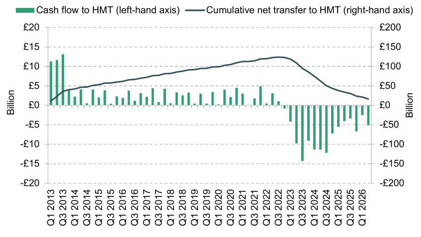
- Since 2009, the Bank of England has bought significant quantities of government bonds, and some corporate bonds, through its quantitative easing (QE) programme. These are held in the Asset Purchase Facility (APF), a legally separate entity which is indemnified by HM Treasury. Between 2009 and 2022, the APF was making profits and a policy choice was made to send these immediately to HM Treasury. These had amounted to £124 billion in total by Q3 2022.
- Since then, the APF has been reducing its holdings (quantitative tightening, QT) and has begun making losses. We estimate that payments from HM Treasury to cover APF losses in 2026–27 will be £19 billion. This is roughly equivalent to total spending on police services in England and Wales. By early next year, the government is expected to have roughly broken even on the QE/QT programme in a narrow accounting sense, but with further losses to come.
- Economic changes since March have increased the APF’s projected losses over the next five years. A higher expectation for Bank Rate increases the cost of financing the loans that initially funded the APF’s bond purchases, and higher yields on government debt decrease the value of the government bonds that the APF decides to sell. The Bank of England also announced changes to the QT programme last month: slowing the pace of bond sales, and concentrating sales on bonds that are set to mature between 2035 and 2049. Together, we estimate that changes since March mean that total APF losses will be around £5 billion higher in each of 2026–27 and 2027–28. Largely as a result of the changes announced by the Bank, total losses are expected to fall to £13 billion in 2030–31 – £6 billion less than we expected in March.
- Only a portion of these losses affect the fiscal aggregates that are targeted by the government’s fiscal rules. We estimate the changes since March are likely to reduce the current budget surplus – revenues net of day-to-day spending – by £3.4 billion. In contrast, we expect them to leave the government’s preferred measure of debt (PSNFL) roughly unchanged in the same year. Importantly, under current arrangements, the whole of any losses results in a cash transfer from HM Treasury to the APF. This can be funded through higher government borrowing, higher taxes or reduced government spending on other things.
- Other ways of managing these losses are possible, and have international precedents. Changing arrangements between HM Treasury and the Bank would not be a free lunch: all options would amount to reallocating losses either through time or between different groups in the economy. However, given the extent of the costs in the near term, now is the time for an open and informed discussion of these arrangements.
4.1 Introduction
In response to the financial crisis of 2008 and subsequent shocks, the Bank of England, along with other global central banks, bought significant quantities of government bonds, in a policy known as quantitative easing (QE). More recently, it has been reversing this through quantitative tightening (QT), allowing its holdings of these bonds to mature without replacing them and actively selling some back to investors on financial markets.
Over the course of this policy, the Bank has made gains and losses, which have resulted in payments to and from HM Treasury. The technical arrangements surrounding this are complex, but they are important, because the exact arrangement affects the government’s fiscal position.
In this chapter, we explain how the QE/QT programme is operating and describe the recent changes announced by the Bank. We discuss how gains and losses currently feed through into transfers to and from HM Treasury and impact the public finances, and how the scale of these transfers is set to change in the coming years. Finally, we discuss whether there are changes the government could make to its arrangements with the Bank which would impact the fiscal arithmetic in the coming months and years.
Box 4.1. How do bonds work?
One way that companies or governments can borrow is by issuing bonds. Effectively this involves selling IOUs for future payments. When issuing a bond, the issuer sets a term (e.g. five years) and can then include commitments to two different types of future payment:a
- a coupon: an amount paid at regular intervals (e.g. every six months) over the life of the bond;
- a redemption value: an amount paid at the end of the bond’s term (at maturity).
For example, a government or company could issue a bond that lasts ten years and promises to provide £5 each year for those years, and a further £100 when it reaches maturity.
When government issues (sells) a bond to a lender, it receives an up-front payment – the price. The price of bonds reflects the balance of demand and supply for that specific type of bond. If lots of investors want to buy a particular type of bond, it might have a high price; if there are low levels of demand relative to supply, it might sell for a low price. The demand and supply for a given bond will depend both on economic conditions, such as central bank policy rates and inflation, and on the specific characteristics of the bond issuer.
The higher the price of a given bond, the lower the effective interest rate – the yield – on that bond. Take a simple example of a bond that only lasts one year, offers no coupons and has a redemption value of £100 after that year. If it is sold for £90, the lender gives up £90 immediately for a promise of £100 a year later. They receive interest of £10, so the effective interest rate is 11% (£10 divided by £90). If instead the same bond sold for £95, the lender would only receive £5 of interest after a year, so the effective interest rate would be 5.3% (£5/£95).
As well as a primary market for bonds – in which lenders buy bonds directly from bond issuers (in this case, government) – there is also a secondary market for bonds. A lender who has already bought a bond can sell it on. In doing so, the original lender receives cash immediately in return for giving up any remaining coupon payments on the bond and the future redemption value.
a In most cases, the coupon and redemption value of a bond are fixed cash amounts. There are also inflation-linked bonds where the value of the coupon payment and the redemption value are automatically uprated with inflation.
4.2 A brief history of quantitative easing and quantitative tightening
Quantitative easing (QE) was rolled out in 2009 during the financial crisis to help stimulate the economy out of recession and bring inflation up to the Bank of England’s 2% target. It was an untested tool and there was limited precedent to inform its design. In order to let the Bank of England focus on its aim of stabilising the economy, rather than concerns of the potential profit and loss inherent in holding a large portfolio, the Bank and the government agreed that the bonds purchased would be held in a legally separate entity rather than directly on the balance sheet of the Bank of England. This entity was termed the Asset Purchase Facility (APF). The government then guaranteed, or indemnified, the financial position of this facility, meaning HM Treasury would make good on any losses that were incurred.
The APF then purchased predominantly government bonds, as well as some corporate bonds, from the market. It funded these purchases with a loan from the Bank of England, on which it is required to pay the Bank of England’s base rate – like a tracker mortgage. The Bank of England in turn financed these loans by creating new money, in the form of reserves held by commercial banks, on which it pays interest at the Bank of England’s base rate.
When QE was initiated, the UK was in recession and inflation was below the Bank’s target, so the Bank wanted to stimulate additional demand in the economy. By buying government and corporate bonds, the APF aimed to reduce interest rates across the economy, reducing the cost of borrowing for both households and firms, with the aim of stimulating additional investment and consumption.
QE was used to support the economy after the 2008 global financial crisis, following the 2016 Brexit shock and in response to the 2020 pandemic-induced slowdown. The APF’s bond holdings peaked in 2021 when it owned £875 billion in gilts (around a third of total government debt) and a further £20 billion in UK corporate bonds (Ramsden, 2023).
QE was always intended to be a temporary intervention. Since 2022, the Bank of England has been ‘unwinding’ it, reducing the stock of bonds it holds in the APF. This has become known as quantitative tightening (QT).
The Bank has carried out QT in two ways. First, it has let some bonds reach maturity. When this happens, the APF receives the redemption value from the bond issuer and pays back the initial loan it took out from the Bank of England. This is termed passive unwind. Second, the Bank has sold some bonds on the market. The APF then receives the going market price for the bond and pays back the initial loan it took out from the Bank of England, which in turn reduces the reserve balance of commercial banks, all else equal. These are called active sales, or active unwind.
4.3 How do QE and QT lead to financial flows between HM Treasury and the Asset Purchase Facility?
There are three direct ways that the QE/QT programme affects the public finances. All of these involve cash flows between HM Treasury and the Bank of England, but they have different effects on the fiscal aggregates (such as measures of government spending and debt).
First, there is the interest rate loss or gain. This is the coupon payments the APF receives for the bonds it owns, minus the interest it pays to the Bank on the loan it used to finance the purchases (on which it is charged Bank Rate). For a long time, the APF was making a profit as the coupon payments it received from its bond holdings averaged 3–4% of their purchase cost and Bank Rate was at rock-bottom levels of 0.5% or less. From 2012 onwards, this interest rate gain was sent each quarter to HM Treasury. The decision to send these profits immediately to HM Treasury was a policy choice; the government and the Bank could instead have agreed to keep those profits within the APF’s portfolio to cover potential future losses.
More recently, this interest rate channel has turned negative. Bank Rate has risen (and is expected to rise further) while the coupon payments on the bonds have remained unchanged. Each quarter, the government sends payments to the APF to cover this loss and these are counted as current or day-to-day spending.
Second, there are maturity losses or gains. These occur when a bond is held until redemption (passive unwind). At this point, the APF receives the redemption value of the bond from the bond issuer (in most cases, the government). This redemption value is often different from the price the APF paid for the bond initially – the initial proceeds amount – and the difference between these two is the maturity loss/gain.
At the point when the APF initially buys the bond, the government can anticipate the future maturity loss (or gain), and so for all bonds purchased the difference between the purchase value and the redemption value is recognised on the government’s balance sheet up front through an adjustment in the level of public sector debt (PSND). This means that when the loss is actually realised when the bond matures, there is no additional shift in PSND or public sector net financial liabilities (PSNFL), an alternative measure of debt.
Third, there are the sales losses or gains. These occur when the APF sells a bond to the market (active unwind) and reflect the difference between the price paid for the bond originally – the initial proceeds amount – and the price at which the bond is sold. Conceptually, this is because the APF receives the current price of the bond from the market, but must pay back a portion of the loan it owes the Bank equal to what it borrowed to buy the bond in the first place. As with maturity losses, this loss does not affect day-to-day government spending in the current budget, but it does add to public sector debt. A key difference is the timing. As the eventual sale price is not known when the APF first buys the bond, the sales gain or loss only adds to PSND and PSNFL in the year the bond is sold.
Where there are losses, the cash transfer to the APF – the sum of these three losses – does have to be funded. It adds, all else equal, to the government’s net cash requirement.
As well as the direct fiscal implications of transfers relating to the QE/QT programme, there are also indirect consequences for the government’s finances. The QE programme increased demand for government bonds and so reduced yields and government borrowing costs, although this was not the primary aim of the policy. The QE programme did aim to stimulate growth, at a time when the UK economy was in recession. Higher growth would also have been positive for the government’s finances. Viewed narrowly, QT acts in reverse on both these same channels. However, the difference for QT is that, with interest rates still a long way from the low levels of the 2010s, the Bank can, and does, look to offset this drag by setting Bank Rate lower than it might otherwise have done, meaning the macroeconomic costs of QT through this channel are likely to be less than the benefits of QE. Any broader evaluation of the fiscal consequences of the programme should take these indirect channels into account.
4.4 How big are these financial flows, and what has changed recently?
Scale of financial flows
Between 2009 and 2022, the APF was making a profit and the cumulative cash flows to HM Treasury peaked at £123.9 billion in Q3 2022.1 Since then, money has flowed back the other way at an average pace of around £30 billion per year. By the end of Q2 2026, the net cumulative flows to the Treasury remained positive, but just, at £16.2 billion: HM Treasury has roughly broken even on the QE/QT programme so far. Continuing losses mean this is likely to turn to a cumulative loss by early next year.
Figure 4.1. Quarterly cash flows from APF to HM Treasury and cumulative value of total transfers from APF to HM Treasury
Source: Barclays Research.
Estimates of the scale of these projected flows in future years are very sensitive to what one assumes about bond yields, Bank Rate, and both the pace and maturity profile of the Bank’s QT programme.
In March, the Office for Budget Responsibility (OBR) assumed that the Bank of England would unwind the APF by actively selling £32 billion of bonds each year, on top of whatever naturally reached maturity.2 On this basis, it projected that losses – and so flows from HM Treasury to the Bank – would average around £19 billion per year over the next five years. This is roughly equivalent to the entire budget for policing in England and Wales.
Recent Bank of England announcements on QT programme
Helpfully, at its annual review of the QT programme in September, the Bank of England resolved much of the uncertainty around this path, publishing a multi-year outline of what it plans to do.3 This gives us greater certainty and allows us to model more confidently what the fiscal flows will be.
The Bank of England explicitly stated it plans to actively sell £20 billion of government bonds each year for the next eight years, £12 billion a year less than the OBR had assumed in March.
Furthermore, it announced that it would not sell any bonds that are set to mature after 2049. Instead, these long-dated bonds will be held and used as a long-term asset to back up the Bank of England’s bank note liability. This matters particularly for the public finances as it is these long-dated bonds which tend to incur the largest losses when sold. It will also refrain from selling any bonds that are set to mature before 2035. These will be held until they naturally mature and passively unwind. This means that all of the sales will be concentrated in bonds that would otherwise mature between 2035 and 2049, as opposed to the previous policy of selling across the entirety of the portfolio.
An important further detail is that, within this 2035–49 bucket, the Bank plans to sell bonds in reverse order of maturity, starting with those with the longest maturity and cascading down. Previously, it had offered all bonds with a maturity of three years left to the market, in buckets of short-dated, medium-dated and long-dated bonds. The precise allocation actually sold then depended on what was demanded by the market.
The final twist in the new phase of QT is that, whereas previously the Bank of England sold bonds to the market, it will now sell them to the Debt Management Office (DMO) – a UK government agency that is responsible for debt and cash management. These sales will still happen at market prices, which means this innovation does little to affect the profit and loss dynamics. But it has the advantage that, by financing these purchases through its normal gilt issuance programme, the DMO can shift the maturity profile of issuance to more closely match market demand.
How have expected flows changed since March?
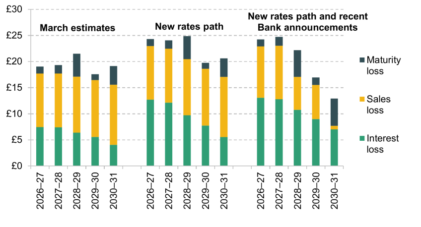
Figure 4.2 compares our estimates for the expected path of flows between HM Treasury and the APF based on the information available in March with our latest estimates of these cash flows.4 Since March, three factors have changed the expected path of flows between HM Treasury and the APF.
Figure 4.2. Estimated APF losses between 2026–27 and 2030–31 under different assumptions
Note: Figures are not adjusted for inflation. March estimates reflect Barclays estimates rather than OBR forecasts.
Source: Barclays Research.
- Expectations for Bank Rate are now significantly higher, as are government bond yields (as we discuss in Chapter 3). Both of these increase the scale of interest rate losses and worsen sales losses. Higher rates increase the spread between Bank Rate and coupons, while higher yields imply lower prices and therefore bigger losses on bonds that are sold. If we model this change in isolation, we estimate it would add £5 billion to losses in 2026–27 and a similar amount in 2027–28, falling to around £1 billion extra in 2030–31. The effect of these changes alone is shown in the second set of bars in Figure 4.2.5
- The new slower pace of unwind of the portfolio, from £32 billion to £20 billion of active sales each year, reduces sales losses in the short term, as fewer bonds are sold and fewer losses crystallised. This is partially offset in future years as slower unwind means interest losses are made on a larger stock of bonds remaining in the APF in future years. Still, the net effect of slower active tightening is to reduce APF losses over the next few years by £3–4 billion per year.
- The Bank of England’s decision to focus sales in the middle segment of its portfolio (to sell only bonds maturing between 2035 and 2049) further reduces the cost of the programme over the life of this parliament as it avoids the APF selling and realising losses on the costliest long-term bonds. However, the decision to sell bonds within this bucket in reverse maturity order adds some of this back in, relative to a scenario in which sales were distributed evenly across maturities in the portfolio. The net of these two adds to APF losses by £3–4 billion over the next two years before falling to be broadly neutral in 2028–29 and 2029–30.
All taken together, our modelling suggests that total cash flows from the government to the APF in each of 2026–27 and 2027–28 are likely to be higher than expected in March. The impact in 2028–29 and 2029–30 is more neutral, with overall flows estimated to be around £6 billion lower in 2030–31 than expected in March.
4.5 How does this affect the public finances?
As mentioned above, the three different types of losses affect various fiscal aggregates differently. This means they have different implications for the government’s compliance with its two main fiscal rules:
Borrowing rule. This rule requires the government to achieve a forecast current budget surplus – with government revenues exceeding day-to-day spending – in the third year of the forecast, currently 2029–30. Of the three cash flows discussed above, only the interest losses count as day-to-day spending so only this one directly affects the government’s compliance with the borrowing rule. We estimate that interest losses will be £9.0 billion in 2029–30 – £3.4 billion higher in 2029–30 than our March-based estimates, reducing the government’s headroom against this rule – all else equal – by £3.4 billion. Of this, we estimate £2.2 billion results from the change in Bank Rate expectations and £1.2 billion from the Bank’s new approach to quantitative tightening.
Debt rule. This rule is a commitment to have the government’s preferred measure of debt, public sector net financial liabilities (PSNFL), falling by 2029–30. This rule is affected both by sales losses – which increase PSNFL in the year they are realised – and interest losses. We estimate that in 2029–30, the sum of the interest and sales losses will be £15.5 billion, £0.9 billion lower than our March estimates.6
Whatever the precise implications for compliance with the fiscal rules on any particular time frame, it is still the case that under current arrangements, the totality of interest, maturity and sales losses needs to be made good and the transfer from HM Treasury to the APF needs to be funded. All else equal, these transfers add to the government’s net cash requirement, increasing the amount of debt the government issues to the market. If government chose to adjust borrowing (rather than taxes or spending on other things), the government would have to borrow an estimated £5.2 billion more from the market in 2026–27 and £5.4 billion more in 2027–28 as a result of changes in forecast APF losses. This is against a backdrop of expected borrowing of around £300 billion per year.7 The impact thereafter is broadly neutral in 2028–29 and 2029–30, and changes since March would actually lower borrowing in 2030–31 by around £6 billion.
4.6 Does the timing of APF losses matter?
Several commentators, including the Governor of the Bank of England, have stated that the precise timing of losses, and how they are accounted for on the combined public sector balance sheet (which brings together the Bank and the government) are simply a matter of accounting and not economically important. On one level, this is true. HM Treasury will ultimately bear the costs of the QE/QT programme. Whether losses are crystallised now through sales or later through maturing bonds should, in the long run, lead to a similar eventual loss, when discounted through time. And given HM Treasury’s commitment to indemnify those losses, whether transfers to the APF are made now or in some future year only moves resources through time.
However, to draw on the often-used sentiment from Keynes, in the long run we are all dead, and if economics is anything, it is the study of how to best allocate our resources not just across people and places, but also across time. Keeping the current arrangements is a choice to spend £20 billion per year on a transfer to the Bank of England now, rather than to do that at some other time. This is a similar choice the government faces when it is deciding whether to bear the costs of public spending now through taxation or to borrow now and finance them through taxation in future. Both choices involve choosing how to distribute costs between current taxpayers and future taxpayers, or between different groups of taxpayers at a given point in time.
4.7 Alternative ways of managing and accounting for the costs of QT going forward
Given the importance of how these flows are distributed across people and time, a number of alternative arrangements have been discussed that would result in a different set of allocations.
One often discussed proposal aims to reduce the near-term costs of the policy by slowing the unwind of the gilt holdings in the APF. As highlighted by the analysis above, this reduces or even removes the sales losses, but elongates both the interest rate losses and maturity losses. In fact, if the entire gilt portfolio were held to maturity, with only passive unwind, HM Treasury would still be covering losses as far into the future as 2071. This problem is particularly acute in the UK compared with its peers as the average maturity of government borrowing in the UK is much longer. This proposal amounts to a shift of the cost burden through time, pushing more of it into the future.
The essence of this proposal has largely been enacted by the Bank of England as part of its September announcement. Although it stopped short of reducing active sales to zero, it reduced the pace of sales and decided to hold a significant fraction of the debt to maturity. One important element of the September decision was that it was led by the Bank of England and motivated through monetary policy and balance sheet management considerations. If the same process had seemed to be dictated by HM Treasury in order to make fiscal savings, this could have been perceived as fiscal policy stepping into the independent decisions of the Bank of England.
A second possible way to reduce the fiscal burden of the APF in coming years would be to reduce the compensation offered on central bank reserves. This is the cost part of the profit and loss equation. If the Bank no longer paid interest on reserves held by commercial banks then there would be scope for the APF to stop paying interest on its loan from the Bank, removing interest losses. Other economies have tried this at a limited scale, reducing the interest they pay on a fraction of the balances held with them in reserves. This change would do nothing to reduce sales or maturity losses, which amount to around half of the overall fiscal burden. This would also effectively shift the loss from government onto commercial banks, who would no longer receive interest income and might pass at least some of the loss on to depositors and borrowers (Islam, Khan and Meaning, 2024). Another risk with this approach would be that it would complicate the implementation of the more traditional tool of monetary policy – the Bank of England being able to set the interest rate on reserves to influence market rates more broadly.8
A third option, put forward previously by one of the authors and others, is that the bonds in the APF could be moved onto the Bank of England’s own balance sheet, removing the government indemnity (Islam, Khan and Meaning, 2024). This is much more in line with how similar programmes have been managed by the Bank of England’s peers in other countries, such as the Federal Reserve. Losses would then have to be borne by the Bank of England, rather than HM Treasury. To deal with this, the Federal Reserve employs a form of accounting known as a deferred asset that allows it to offset current losses with future income streams from the interest on its holdings (seigniorage income).9 Using this internationally established framework would require allowing the Bank to keep its seigniorage income. The framework would allow the Bank of England to smooth out the losses over a longer period. Rather than £20 billion per year over the next few years, the fiscal cost would be more like £1–2 billion per year of lost seigniorage income,10 but these losses would persist over a longer period of time.
4.8 Conclusion
Accounting arrangements between the Bank of England and HM Treasury may seem obscure and complex, but they matter directly for fiscal policy and the decisions that will face the Chancellor, at this Budget and beyond. After years of profiting from the Bank of England’s quantitative easing programme, since 2022 the government has been financing losses. In 2026, this is set to cost £13 billion in interest costs (which represent day-to-day spending for the government) and a further £11 billion in costs relating to the reduction in bond holdings.
Recent innovations from the Bank of England go some way to ameliorate this cost in coming years, but our modelling suggests the OBR will still revise up its projections for these costs in its October forecast. Different countries have chosen different ways of accounting for similar losses and, given the scale of the transfers involved, there should be an open debate about the different options here. This could perhaps be facilitated by the current Treasury Select Committee inquiry into the independence framework of the Bank.
References
Bank of England, 2026. Asset Purchase Facility Quarterly Report - 2026 Q2. https://www.bankofengland.co.uk/asset-purchase-facility/2026/2026-q2.
Islam, M., Khan, A. and Meaning, J., 2024. APF shift: reducing the fiscal burden of QE without tiering. Barclays Research, https://live.barcap.com/go/publications/link?contentPubID=FC6682d38e3b14fb644597c498.
Ramsden, D., 2023. Quantitative tightening: the story so far. Speech, Bank of England, https://www.bankofengland.co.uk/speech/2023/july/dave-ramsden-speech-on-quantitative-tightening-chaired-by-money-macro-and-finance-society.
Ramsden, D., 2026. Quantitative tightening: the next chapter. Speech, Bank of England, https://www.bankofengland.co.uk/speech/2026/september/dave-ramsden-speech-on-quantitative-tightening.
Tucker, P., 2022. Quantitative easing, monetary policy implementation, and the public finances. IFS Green Budget 2022, https://ifs.org.uk/publications/quantitative-easing-monetary-policy-implementation-and-public-finances.
Acknowledgements
This chapter has been produced as part of the IFS Green Budget 2026. It is by authors from Barclays, who have written specific chapters for the 2026 Green Budget, covering topics (the macroeconomic outlook, bond market and Asset Purchase Facility) where their expertise complements that of IFS.
The 2026 edition of the IFS Green Budget is funded by the Nuffield Foundation, Barclays and the Economic and Social Research Council (ESRC) through the Centre for Microeconomic Analysis of Public Policy (CPP). IFS is an independent Research Institute.
Endnotes
Authors

Jack Meaning

Cian Hennigan
More from IFS
Understand this issue


Policy analysis


Academic research