Quantitative easing, monetary policy implementation, and the public finances

Paul Tucker (Harvard Kennedy School)¹ ,²

Key findings

1. Now that interest rates are rising, the interaction of quantitative easing (QE) with the Bank of England’s current methods for implementing monetary policy will add to strains on the public finances. These could, and arguably should, have been avoided by prompt, forward-looking action from around 2019 when the materiality of the risk became apparent (Section 7.2 of main text). As of now, however, there are no easy options. 

2. The crux is that QE creates money that goes onto banks’ balances (reserves) at the Bank of England, and those reserves are being fully remunerated at the central bank’s policy rate (Bank Rate). Given the outstanding stock of QE (£838 billion), that has effectively shifted a large fraction of UK government debt from fixed-rate borrowing (where debt-servicing costs are ‘locked in’) to floating-rate borrowing (where debt-servicing costs rise and fall with Bank Rate). Increases in Bank Rate therefore lead immediately to higher debt-servicing costs for the government, leaving the British state with a large risk exposure to rising interest rates. That exposure is not technically necessary to operate monetary policy effectively, so the predicament was not unavoidable.

3. Stepping back, it is a long-standing principle of the UK’s macro-finance framework that government debt management should not impair the effectiveness of the Bank of England’s monetary policy. It would be sensible to add a new precept: that when, in terms of the objectives for monetary-system stability, the Bank of England is indifferent between options for how to implement its monetary policy decisions, it should opt for methods that interfere least with government choices about the structure of the public debt.

4. That high-level principle points towards the Bank reforming the way it operates its system of reserves. In particular, change would be warranted for how the regime operates in circumstances where, because the Bank is conducting QE, the banks cannot choose the level of reserves each wants to hold, but the extra reserves do not squeeze out their investing in other assets. Under those conditions, the principle implies that the Bank should not remunerate the totality of reserves at Bank Rate but only an amount necessary to establish its policy rate in the money markets. In other words, taken on its own, the principle supports the Bank moving to a system of tiered remuneration for reserves balances, combining no (or low) remuneration for some large portion of reserves with a so-called corridor system acting on marginal reserves to establish the Bank’s policy rate in the money markets (explained in Sections 7.4 and 7.5).

5. Such a change would have considerable benefits for the public purse. Given the Bank currently holds around £800 billion of gilts, Britain’s debt-servicing costs are highly sensitive to even small changes in the path of Bank Rate (Section 7.3). Taking current (6 October) market expectations for a substantial rise in Bank Rate together with the Bank’s current published plans for unwinding QE, the implied savings would be between around £30 billion and £45 billion over each of the next two financial years. These are big numbers, and would of course be even bigger if the Bank does not actively unwind QE via asset sales but lets it roll off as bonds mature

6. Assuming the Bank does go ahead with asset sales, the projected savings from moving to a tiered-reserves regime amount to approximately 1.6% of GDP in 2023–24 and 1.2% in 2024–25 (using Chapter 2’s Citi forecasts). They would, therefore, reduce prospective annual debt-servicing costs from around 3.9% to around 2.3% of forecast GDP in the first year, and from around 2.7% to 1.5% in the second (using Chapter 3’s IFS forecasts). Put another way, if not implemented, the forgone annual saving of (on average) £37 billion over the next few years would be equivalent to around 9% of recent annual spending on health, education and defence.

7. What might seem at first sight like an obvious easy-win reform needs, however, to be balanced against a number of other important considerations. They concern the effects of bank taxes on allocative efficiency, and on credit conditions (Section 7.6); and, separately, central bank credibility (Section 7.7). 

8.  The first and second of those arise because the counterpart to the state’s debt interest savings would be lower interest payments from the Bank to the banking industry on its reserves balances. This could be regarded as a tax on banking and one, moreover, that might depart from standard public-finance-economics prescriptions on the tax system not distorting incentives and being stable over time. The broad point – and the key high-level trade-off – is that in deciding whether to ask the Bank to consider moving to a tiered-reserves system, the government would have to balance, on the one hand, suboptimal taxes being imposed today (to avoid the higher borrowing brought about by a suboptimal debt structure) and, on the other hand, accepting higher borrowing today (to avoid imposing inefficient taxes) and accepting the prospect of having in the future to impose higher taxes (on incomes and consumption) and/or cut the provision of public services. Broadly, this pitches microeconomic considerations against macroeconomic ones. 

9. The standard prescription would be to accept the latter course: do not introduce inefficient taxes when better solutions can be applied over time to the macro problem. The better choice might, however, be affected by whether, in current and prospective circumstances, government might have to pay a default-risk premium on bond-market borrowing unless it cuts the near-term deficit; and by whether more broad-based tax increases and/or cuts in public services are politically infeasible or socially undesirable. 

10. There is also a question of whether a tiered-reserves scheme is best regarded as introducing a tax on banking intermediation or, alternatively, as withdrawing a transfer to banks’ equity holders and managers; crudely, a distinction between banking and bankers. If competitive conditions in banking are such that, as Bank Rate rises, the benefits of fully remunerated reserves would be passed on to neither depositors nor borrowers, but instead would go straight into banks’ profits, then perhaps full remuneration of reserves is better regarded as a transfer. But even if UK banking were uncompetitive (on which we do not take a view), it does not follow that there would be no (or only small) pass-through of higher Bank Rate to banks’ customers. 

11. Quite apart from government needing to weigh allocative efficiency in the economy against its debt burden, the Bank of England would separately need to form its own view on whether withdrawing a flow of income from reserves would hurt the resilience of the banking system; and also whether the macroeconomic effects of any tightening in loan conditions could be offset by monetary policy. 

12. In addition, the authorities would need to weigh some political economy risks. One is the possibility that unremunerated reserves would make QE an attractive source of funding for government, which might warrant higher hurdles in the way of routine monetary financing. Another is that changes in the reserves regime might dent perceptions that the Bank’s operating framework will be stable over time, so any new regime needs to be designed to work well in many different states of the world. 

13. Given the need to balance many different considerations, and given the Bank has private information on the state and choices of the banks, this chapter falls short of recommending that the reserves regime be changed right now. But nor does it rule out early reforms. It is clear, moreover, that, unless the Treasury objects on tax efficiency grounds, the Bank should set out how it will operate a reformed system in future. The prospect of the current predicament recurring is not hypothetical. Given many current estimates of the equilibrium global real rate of interest are close to zero, the lower bound for the UK’s Bank Rate is likely to bite, and so QE be deployed, much more frequently than when the UK’s current monetary policy regime was established. 

14. Finally, the broad principle discussed above – that the Bank should, where consistent with its mandate, adopt methods of monetary policy implementation that interfere least with public debt management – might be thought also to have some bearing on how the Monetary Policy Committee (MPC) chooses to tighten monetary conditions to get control of inflation. Specifically, if the authorities believe gilt yields currently incorporate a default-risk premium but that it will unwind, it might be argued that, on debt-management grounds, the MPC should defer selling gilts (quantitative tightening, or QT) in order to avoid the state paying the risk premium for the residual term of the sold bonds, instead relying entirely on raising Bank Rate to deliver its price stability objective. We believe, however, that the better conclusion is that if the authorities did want to avoid locking in such costs, any adjustment in the pattern of government funding should come in the maturity structure of new issuance by the UK’s Debt Management Office. 

15. That being so, it is important that the significance of this chapter’s central dilemma – between the debt burden and allocative efficiency – would be reduced by early QT sales, since they would shrink the quantum of reserves held by banks with the Bank (whether or not the reserves scheme is reformed).

16. In conclusion, if, as argued here, the Bank’s monetary techniques have distorted the British state’s debt structure in unfortunate ways, it matters that the simplest remedy might introduce tax-induced distortions to the allocation of resources. Balancing those conflicting considerations in current circumstances is a weighty matter for government. This chapter aims to frame the debate. If, having balanced the different considerations, the government were to ask the Bank to consider whether reforms could be introduced without compromising monetary policy, we believe the Bank would need carefully to analyse, and consult on, the implications for price and financial stability. But subject to the government exercising a veto on inefficient-tax grounds, we are not ruling out reforms to the reserves regime for periods when QE is being deployed. 

7.1 Introduction 

There has been growing concern about the effect on the public finances of the government having effectively borrowed at a floating rate of interest, which will increase, possibly sharply, as the Bank of England tries to bring inflation under control. Higher debt-servicing costs would increase government borrowing, and would imply, eventually, some combination of higher taxes and lower spending on public services and other things. This predicament is a complicated product of low equilibrium market interest rates, the authorities’ resorting to quantitative easing (QE) as a substitute for interest rate cuts at the zero lower bound, and central banks paying interest on banks’ reserves. That cocktail of technicalities needs some slow-motion unpacking in order to expose the nature of the problem and the pros and cons of various possible solutions. This chapter aims to do that.

To begin with a sweeping summary, we can say the following. When a central bank purchases government bonds, it leaves the size of the state’s consolidated balance sheet (see annex for definitions) unchanged, but alters the composition of its liabilities. When the central bank pays interest on the money it created to buy those bonds, it changes the profile of interest payments on the state’s consolidated debt, which might turn out to be costly, cheap or neither. There are good reasons to think that UK government debt-servicing costs will be much higher than they otherwise could have been, plausibly running into many tens of billions of pounds.³  While this has become more obvious since the Bank of England’s policy rate started rising, the risk existed even during the period when QE was running a profit (because the policy rate was very close to zero). Proposals for reform have included the Bank of England stopping paying interest on banks’ reserves, and government partially hedging the exposure. In order to explain what is going on, it is necessary to look at the mechanics and economics of how QE interacts with public debt management, the economics of various options for attenuating the link, and some of the background political economy dilemmas. 

From a macroeconomic-policy perspective, a lesson that emerges for the future is that when a central bank’s monetary policy significantly employs QE, it should not remunerate all the reserves held by the private sector but only whatever fraction of reserves needs to be remunerated to establish its policy rate in the short-term money markets. Even if there were reasons to hold back from immediate reform, this implies reforming the Bank’s operating regime after the current stock of QE has unwound but before QE is employed again. But a series of microeconomic policy considerations, belonging more to the Treasury than the Bank, also need to be weighed. So the issue is not straightforward, but it is big – because the implications for government borrowing are big.

The chapter begins with how the risk exposure in the public finances has arisen and in what circumstances it matters (Section 7.2), followed by a range of estimates of the exposure’s quantitative significance (Section 7.3). It goes on to explain why central banks moved to paying interest on reserves (Section 7.4), and whether the current set-up is the only one that can reconcile quantitative easing with control over short-term interest rates (to jump ahead: no). It then outlines, for purposes of exposition rather than recommendation, how monetary policy might operate if interest were not paid on the bulk of reserves (Section 7.5). Having explained the obvious attractions of reforming the Bank’s reserves regime, the chapter turns to microeconomic considerations, setting out some that would need to be carefully weighed against any more macro benefits to the public purse. These concern the effect of taxing banking on the efficient allocation of resources, and on pass-through to customer loan and deposit rates (Section 7.6); and, separately, central bank credibility (Section 7.7). Before concluding, two alternative strategies are briefly noted: hedging part of the exposure, and the Bank relying on selling off its gilt portfolio, rather than increasing its policy rate, when it wishes to tighten monetary conditions (Section 7.8). After recapping how its main findings relate to public risk management and accountability, the chapter draws to a close by suggesting a new principle to help guide the interaction of monetary policy and public debt management.

7.2 Central banking and the public finances: qualitative analysis

Central banks’ financial operations affect their countries’ public finances in a very direct way. A central bank is a machine for issuing the money that is the final settlement asset in a monetary economy – known to economists as base money (see annex). It alters the amount of this money circulating in the economy via financial operations of various kinds. Those operations change the structure and/or size of the state’s consolidated balance sheet.

If a central bank buys only government paper, the structure of the state’s consolidated liabilities is altered, but its size is left unchanged because one organ of the state (the central bank) has bought the liabilities of another (central government). Monetary liabilities are substituted for government’s longer-term debt obligations. If, by contrast, the central bank purchases private sector paper or lends secured or unsecured to the private sector, the size of the state’s consolidated balance sheet increases, with monetary liabilities being added to the government’s outstanding debt, and in addition the risk structure of the state’s consolidated asset portfolio shifts.⁴

In each case, it matters whether the central bank pays any interest on its monetary liabilities, and at what rate of interest. For around 20 years (as explained in Section 7.4), the main central banks have paid interest at or close to their policy rate on reserves balances held by banks; the Bank of England pays its policy rate, known as Bank Rate (defined in the annex, and shown for the period since Bank of England independence in Figure 7.1). In consequence, when the central bank purchases government bonds – via what is known as quantitative easing or QE – there is an effect on the public finances. Whatever its utility for monetary policy (not discussed here), the combination of QE and interest-on-reserves is roughly equivalent, for the public finances, to the Treasury department entering into a debt swap with the private sector via which fixed-rate government debt is swapped for floating-rate obligations. This means that rather than locking in the rate of interest it pays to borrow, the state pays a rate of interest that is reset each time – roughly every six weeks – the Bank of England decides its policy rate, and so goes up or down when Bank Rate goes up or down.

For the UK, so long as the state’s sovereign creditworthiness is not in question, the implications for the public finances of long-lived QE are most easily examined in terms of the state’s expected and realised debt-servicing costs (i.e. ex ante and ex post) rather than any volatility in the mark-to-market value of the QE gilt portfolio.⁵  The state is not liquidity constrained – not least because the Bank can create money provided it maintains credibility for low and stable inflation – so the state can finance itself through any nasty volatility in the value of its asset portfolio.⁶  Until and unless QE is unwound by selling bonds (Section 7.8), the state’s notional mark-to-market gains and losses are typically not realised because, ordinarily, government does not trade in its own debt or buy back bonds before maturity. 

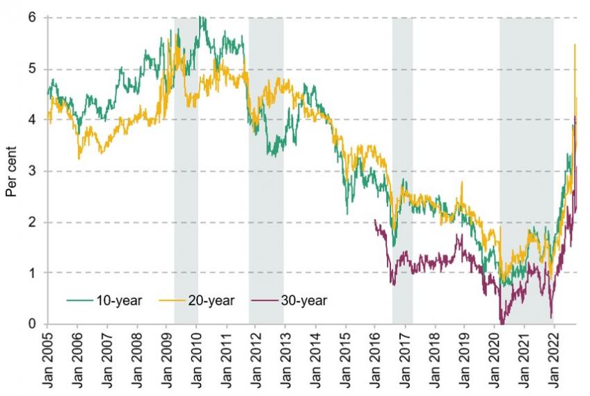
Figure 7.1. Bank Rate since Bank of England independence

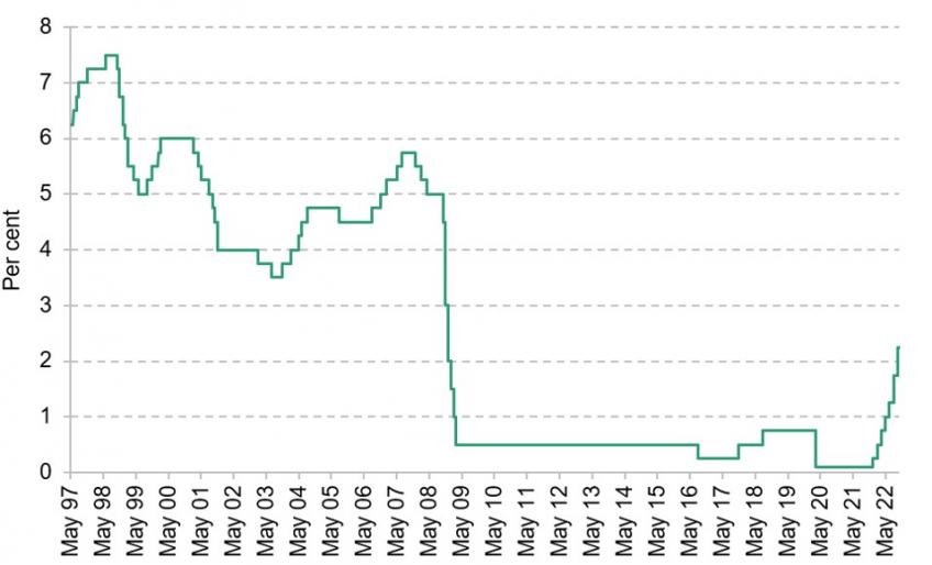
Source: Bank of England.

While this can be obscured by the complex arrangements between the Bank and HM Government (HMG) for conducting QE – involving an Asset Purchase Facility (APF) booked to a special purpose vehicle, an indemnity and other things (Box 7.1) – what matters to taxpayers is the position where Bank–HMG transfers are netted out, leaving only the state’s net transactions with the market. By introducing a couple of simplifications, this becomes clear. If we assume that the Bank holds the gilts it buys until maturity and that it buys new gilts at the yield at which they were issued into the market (a reasonable approximation for 2020–21),⁷  the financial effect of QE on the state’s ex post debt-servicing costs – positive or negative – is simply equal to the Bank’s cumulative profit or loss from buying and holding a long-term bond and financing it by borrowing at Bank Rate. If, therefore, over the life of the bond, Bank Rate averages the yield at which the bond was issued (and purchased), QE does not materially affect the public finances. If Bank Rate is on average higher than that yield, the Bank makes a loss, which it passes on to the Treasury, and so the state would have financed itself more cheaply if the Bank had not bought the bond. Conversely, the state saves money if Bank Rate averages below the yield on the bond.⁸

Box 7.1. The Asset Purchase Facility vehicle

The Bank of England implements QE via a special purpose vehicle called the Bank of England Asset Purchase Facility Fund Limited (APFF Ltd). The company is a fully-owned subsidiary of the Bank. 

When the vehicle purchases gilts, it finances the purchases by borrowing from the Bank’s Banking Department, which charges a rate of interest set at Bank Rate. The reserves created are liabilities of Banking Department. So in double-entry bookkeeping terms, Banking Department’s liabilities increase by the amount of reserves created and held by banks, and its assets increase by a loan to APFF Ltd of exactly that amount. Both liabilities and assets pay Bank Rate, so Banking Department has no interest-rate exposure.

Meanwhile, APFF Ltd has a debt liability to Banking Department costing Bank Rate, and assets comprising the gilts bought as part of the QE operations. The APFF Ltd therefore has an exposure to interest rate risk: it has borrowed at a floating rate, and invested in a portfolio of fixed-rate securities. The Treasury indemnifies APFF Ltd against any losses incurred via that exposure, and it receives any running profits (when Bank Rate is lower than the average yield on the APF portfolio). (a) It was initially envisaged that there would be a settlement of any profits or losses at the end of the QE scheme. But in late 2012 it was announced that quarterly cash settlements would be introduced as QE was not winding up on anything like the timescale envisaged. (b)

Securities bought and held by the vehicle are, for accounting purposes, marked to market (MTM). Any MTM gains or losses are offset by changes in the accounting value of amounts due to or from the Treasury under the HMT Indemnity since that too is valued on an MTM basis (note 8 to BEAPFF 2020–21 accounts).

Figure 7.2. Cash flows to and from the Asset Purchase Facility

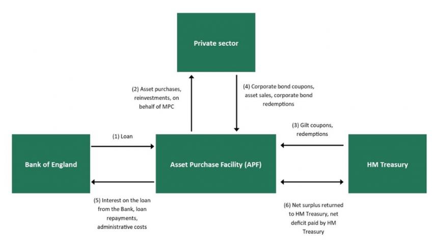
Source: Adapted from Bank of England, Cash transfers between BEAPFF and HMT, https://www.bankofengland.co.uk/-/media/boe/files/markets/asset-purchase-facility/cash-transfers.pdf.

(a) The indemnity is best thought of as an instrument of political economy designed to make clear up front to everyone, including parliament and the public, that any Bank losses would fall on the Treasury. In fact, under the UK system, that would have been so anyway, but might not have been widely understood.

(b) Confirmed on page 4 of the BEAPFF Annual Report and Accounts for 2020–21. Quarterly cash settlement mirrors long-standing arrangements for the Bank’s Issue Department (to which pound-note liabilities are booked). The Bank was split into Issue Department and Banking Department in 1844 by legislation introduced by Prime Minister Peel.

The risk exposure

As the above makes clear, since QE combined with remunerated reserves shifts the state’s consolidated liability structure, it obviously alters its exposure to risk, where risk is conceived of as uncertainty about the path and the net present value of the state’s debt-servicing costs. The incremental risk exposure is greater the larger the stock of QE, and risks are more likely to crystallise the longer the exposure lasts. In fact, of course, QE has ended up being very much larger and much longer-lasting than envisaged back in 2009–10. The stock of QE rose from £200 billion at end-2010 to £435 billion at end-2019 and £875 billion at end-2021 (Figure 7.3).⁹

Figure 7.3. Cumulative gilt purchases via the Bank of England Asset Purchase Facility

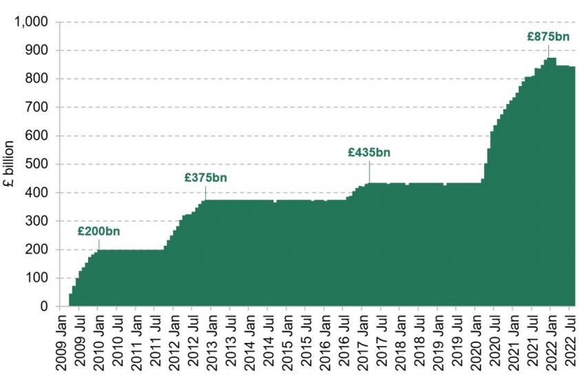
Note: Figures show purchases of gilts only and exclude approximately £20 billion of corporate bonds purchased by the APF. 
Source: Office for National Statistics series FZIU (BoE: Asset Purchase Facility: total gilt purchases: £m CPNSA).

It is natural to think of the risk exposure in terms of the uncertainty that arises from the structure of the state’s debt stock veering away from what analysis had suggested would be sensible absent QE. Had fiscal stimulus, not monetary stimulus, been the favoured instrument for promoting economic recovery from the middle of the 2010s, the annual deficits would have been larger but the structure of the state’s debt would presumably have been broadly unchanged (given a stable debt-management strategy for many years).

Government’s choice of debt structure in normal conditions should be based on analyses of the pattern of shocks – their type and possible scale – that might plausibly hit the economy. That entails assessing the prospective effects on tax revenues and spending of a wide range of shocks, taking account of whether different types of gilt issuance provide insurance to the private sector and so dampen or amplify the transmission of shocks. Given the shocks might be nominal (e.g. to the credibility of the monetary regime) or real, and that those real shocks might be to demand (e.g. to consumer tastes) or supply (e.g. to technology), and sourced either domestically or externally (notably, an energy price shock), the standard choice – certainly in the UK – is to issue both nominal bonds and inflation-indexed bonds spread across the maturity spectrum.¹⁰ More plainly, it makes sense to avoid effectively betting, via a lopsided debt structure, on certain types of shock never occurring.

That, in its direct effects, is what swapping the debt into floating-rate nominal liabilities amounts to for the public finances. The Bank of England’s QE operations purchased only nominal bonds, not inflation-indexed bonds.¹¹ From the perspective of debt management, those purchases accordingly undid HMG’s favoured duration choices for nominal issuance, while leaving the nominal/indexed split of the public debt unchanged. This meant, among other things, that in the face of a positive shock to domestically generated inflation that monetary policy did not pre-emptively offset, debt-servicing costs would be hit by both a permanent increase in the cost of servicing inflation-indexed bonds, and a temporary increase in the Bank Rate paid on reserves when monetary policymakers caught up (a risk that is crystallising currently). We assume here that the authorities were right to exclude inflation-indexed bonds from QE as that left the British state with its (deliberate) exposure to rises in inflation, and so left intact the incentives for the Treasury to favour low and stable inflation, and thus to maintain a strong, independent central bank that can control domestically generated inflation (see Section 7.7).¹²  The QE-induced risk exposure that matters, therefore, concerns only the state’s consolidated nominal debt.

When does the risk exposure matter?

Whether the risk exposure matters, however, turns on more than probabilities, as a risk could crystallise but be immaterial in its effects. Here things are a bit more subtle. Qualitatively, the exposure does not greatly matter ex ante if the plausible possible paths for Bank Rate all average around the plausible range for yields on medium-to-longer-term gilts, or ex post if Bank Rate is not on average materially higher than the yields at which gilts were issued before being bought by the Bank. As explained above, if those conditions are met then temporary divergences of Bank Rate away from its expected path are not going to make much difference to the state’s funding costs relative to the counterfactual of government financing itself in the market (provided, as already stated, that fiscal credibility is solid). 

In the ordinary course of things (assuming fiscal credibility), long-term bond yields would reflect the expected path of the short rate, plus a so-called term premium to compensate investors for locking up their funds (and assuming market-risk exposure if they might sell before maturity).¹³  When the expected path of policy rates is low (and the supply of long-maturity gilts does not stretch demand), that term premium might be compressed because more asset managers will try to enhance the returns on their investment portfolio by earning the illiquidity premium (one of many manifestations of the proverbial search for yield). 

That means that one reasonable indicator of the materiality of the risk exposure, ex ante, is whether or not the long-term forward rate of interest (see annex) is roughly – in a plausible range for – what people think will be the steady-state nominal rate of interest (roughly, Bank Rate). Figure 7.4 shows the evolution over time of the 10-, 20- and 30-year forward rates for the 12-month nominal rate of interest. It shows that in 2009 and 2010 when QE began, the long-run forward rate was still around 5%, which is broadly consistent with inflation averaging 2% and the real return on (roughly) risk-free assets averaging 2–3% over the long run. As such, the risk exposure initially opened up by QE was not obviously material on this count, since borrowing at a fixed long-term rate could be expected to be around the average of Bank Rate over the life of a long-term bond.¹⁴

Figure 7.4. Nominal 10-, 20- and 30-year forward rates, January 2005 to present

Note: Data run to 6 October 2022. Shaded areas indicate periods when the Bank of England was undertaking quantitative easing and purchasing gilts via the Asset Purchase Facility. Data for 30-year forward rates unavailable prior to 2016. 
Source: Bank of England.

By mid-to-late 2019 – notably, before the 2020 COVID-19 pandemic began – long forward rates were unusually low: the 20-year forward rate was between 1% and 2%, and the 30-year between 0% and 1%. Subject to one caveat, this implies that, ex ante, it would have been much cheaper to fund the government by issuing long-term bonds to the market, thereby locking in the unusually low long forward rates, than by borrowing at a floating rate from the Bank of England. That is because Bank Rate would have been expected to be higher over the life of the bond than the long forward rate. The caveat is that that inference would not hold for anyone who, at the time, had an extraordinarily pessimistic view of the outlook for growth (and, therefore, the return on capital), and/or thought inflation would systematically undershoot the prevailing 2% target. There is no evidence (we know of) that the authorities held either view, let alone both.¹⁵

Figure 7.5. Nominal 10-, 20- and 30-year forward rates, 1 September 2022 to present

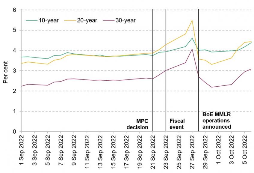
Note: Data run to 6 October 2022. Vertical lines indicate the MPC’s 21 September announcement, the Chancellor’s 23 September fiscal event, and the start, on 28 September, of the Bank of England’s market-maker-of-last-resort (MMLR) temporary gilt purchases. 
Source: Bank of England.

There is also another contrast between the 2009–10 and 2020–21 episodes of QE. During the former, in the aftermath of the financial crisis, there was slack in the economy, and thus no meaningful prospect of domestically generated inflation requiring a period of tight monetary policy. In consequence, the Monetary Policy Committee (MPC) was in a position to accommodate various cost shocks that hit the UK during 2010–11. In the later period, by contrast, it was harder to be so confident about domestically generated inflation pressures remaining muted given persistent additions to monetary stimulus and, following COVID, a large number of people withdrawing from the workforce (reducing the economy’s productive capacity) – even before Russia’s war on Ukraine and the various resulting cost shocks. As it turned out, that risk seems to have crystallised, implying a period of tight monetary policy during which Bank Rate will be above its expected long-run average. In other words, the public-finance risk exposure created by floating-rate funding through 2020 and 2021 was exacerbated by a non-negligible chance of an inflationary shock. The point is not that this should certainly have been the expected outcome, but that it was a meaningful possibility – the risks to inflation were regarded by some as plainly to the upside – raising the stakes of adding to QE.

Summing up, it is reasonable to conclude that by the autumn of 2019 it was clear there was meaningful risk to the public finances from the combination of QE and paying interest on banks’ reserves.

7.3 Quantifying the opportunity costs and risk exposure

Materiality in the probability of a risk crystallising and materiality in the costs of its crystallising are obviously not the same thing. This section aims to put some numbers around the opportunity costs and continuing risk exposure by looking at, in turn, the what-if of QE having stopped before 2020, the sensitivity of funding costs to the path of Bank Rate, and the savings available if interest was no longer paid on banks’ reserves.

Opportunity costs from funding via QE over 2020–21

An obvious place to begin, given the previous subsection, is to put some numbers on the savings that might have been secured had the Bank not added to its QE after 2019, when it became clear long-run forward rates of interest were unusually low. This involves assuming, counterfactually, that throughout 2020 and 2021 the government borrowed in fixed-income markets (without any fixed-to-floating debt swap) to fund the fiscal assistance provided to the country during the pandemic, and that the Bank chose not to buy-and-hold more gilts.

The Bank of England bought £440 billion of gilts during that period.¹⁶  To simplify things, one plausible benchmark is to assume that, instead of QE, the government funded in the market at the average yield over that period at the average duration of the conventional part of debt portfolio (ignoring QE), which was approximately 12 years.¹⁷ Assuming no effect on borrowing costs (see below), the interest rate incurred would have been approximately 0.7%.¹⁸ In fact, a respectable case could have been made for the government lengthening the duration of issuance during this period to take advantage of the unusually low long-maturity forward rates, but that is ignored here.¹⁹

In the short run, funding via gilt issuance would have been more expensive than funding via QE at Bank Rate, which averaged 0.17% over the period from 1 January 2020 to 31 December 2021. But things were set to turn round once Bank Rate was returning back to something like neutral. Taking the Bank’s recent estimate of the steady-state equilibrium nominal rate of interest of 2% (and assuming no change in the outstanding amount of QE),²⁰ the annual savings would in steady state have been roughly 1.3% (on the £440 billion of gilts), or £6 billion per year. If, instead, the equilibrium nominal rate were, say, 3% (roughly the 20-year nominal forward rate in late August 2022, so before the recent fiscal-event shock), the steady-state savings would have been nearly double: roughly 2.3%, or £10 billion per year. Using 2021–22 numbers for national income, those steady-state savings would be around 0.2–0.4% of GDP per year, or 0.5–1.0% of total government spending. If instead the equilibrium were 4.4% (the 20-year nominal forward rate at the time of writing, 6 October – see Figure 7.5), the steady-state savings would rise to 3.7%, £16 billion per year, equivalent to 0.7% and 1.5% of 2021–22 GDP and total government spending, respectively. 

Those numbers assumed that if HMG had funded itself in the markets during 2020 and 2021, that would not have affected yields. But long-maturity nominal forward rates were so low then that the supply effect on yields would have had to have been in the order of 1–2 percentage points for the implied steady-state saving to be wiped out. At the least, it can be argued that, monetary policy considerations aside (see Assessment subsection below), government could usefully have tested the waters rather than relying on Bank purchases.²¹

Forward-looking risk analysis: the Office for Budget Responsibility’s reports

That was backward-looking: assuming different policy choices on QE had been made over recent years. Taking recent policy towards QE and reserves as given, the Office for Budget Responsibility (OBR) has published two reports containing forward-looking analyses of the risk to the public finances from the UK state’s de facto fixed-to-floating debt swap.²² They approach this by observing that the Bank’s operations have considerably shortened the average duration of the debt stock. They calculate the reduction in the mean duration; and also, given that the mean is lengthened by a few very-long-maturity bonds, in the median duration, which serves, OBR points out, as ‘a direct measure of the time it takes for half of the full effect of a rise in rates to feed through to interest payments’. In March 2021, the OBR reported that whereas the median maturity of the government’s total gilt liabilities excluding the Bank’s APF was around 11 years, it fell to 4 years if the APF was included. This meant that (as of March 2021) 59% of the government’s debt liabilities would respond to changes in interest rates over the (five-year) forecast period, compared with 44% in early 2009 (prior to QE). Relatedly, a 1 percentage point increase in short rates was estimated to increase debt interest spending in the final year of the forecast by three times as much as in December 2012: some 0.45% of national income (equivalent to more than £11 billion in today’s terms), versus 0.16%.²³

The OBR has also explored the effect on debt-servicing costs of scenarios where the long-run equilibrium real rate of interest (known as R*) rises with and without an equivalent increase in the underlying rate of economic growth. Inflation is assumed to be at target, because the Bank is assumed to anticipate the shocks. Obviously, the debt-to-GDP ratio rises when the equilibrium real interest rate rises without a corresponding increase in growth. In its July 2022 analysis, the OBR found that a permanent 1 percentage point increase in gilt yields without any change in economic growth would, over a 50-year horizon, increase the ratio of debt to GDP by around 60 percentage points (from around 265% to around 325% of GDP).²⁴

These are important, useful thought experiments, but they do not exhaust the range of scenarios where a reduction in the effective duration of the state’s consolidated debt proves costly. In part, this is because the reduction in the debt stock’s median duration is not an adequate summary statistic for the changes brought about by QE to the state’s debt structure. In principle, a borrower could have a median debt duration of three years without having any debt that repriced every month, and so without being sensitive to sharp but temporary shifts in the monetary policy rate.

Figure 7.6. Overnight Index Swaps forward curve (short end)

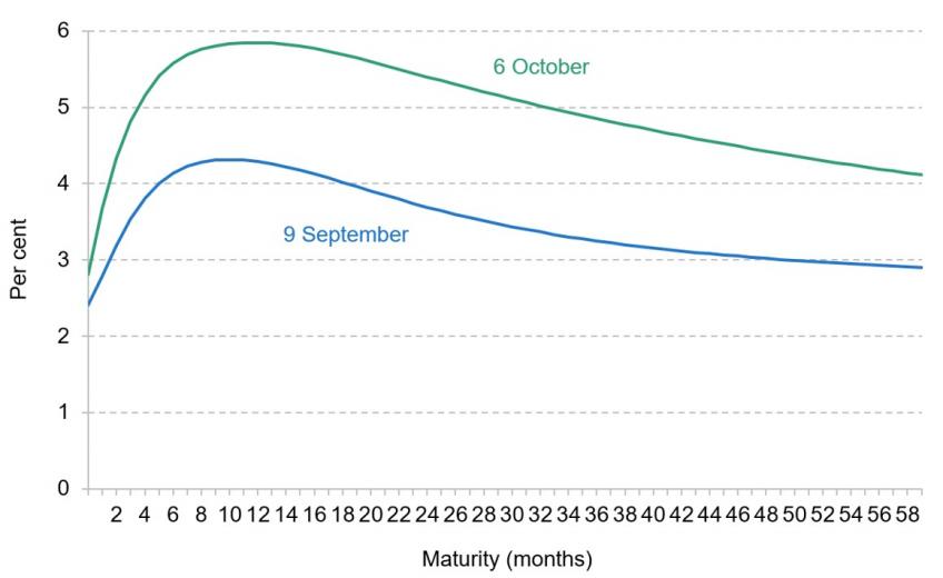
Source: Bank of England.

Figure 7.7. Overnight Index Swaps forward curve

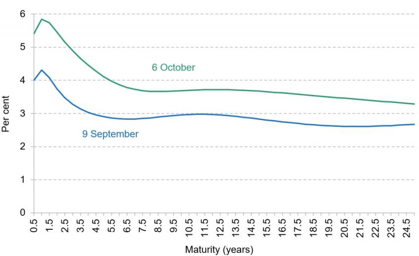
Source: Bank of England.

In terms of illustrating the state’s risk exposure via scenario analysis, the point is that a permanent shift in the long-run equilibrium real rate of interest without higher growth does not exhaust the set of unpleasant scenarios. Another important scenario, as suggested in the previous section, was, hypothetically, of a temporary sharp increase in Bank Rate in order to bring domestically generated inflation back under control or to re-anchor medium-term inflation expectations. Given the British state’s floating-rate debt, a temporary monetary policy shock of that kind would, while it lasted, increase debt-servicing costs while temporarily pushing GDP below the path that would have been sustainable in the absence of the inflationary shock. A variant of that shock has, of course, occurred – initially as underlying inflationary pressures became apparent to financial-market participants, and intensifying after the fiscal event of 23 September. Taking the current (6 October) market-implied path for Bank Rate (shown in Figures 7.6 and 7.7) and the Bank’s announced plans for unwinding QE,²⁵ the cost of servicing the QE-related debt (at Bank Rate) would be £90 billion between now (October 2022) and March 2025 (£42 billion and £33 billion in each of the next two financial years).²⁶ ,²⁷ We return to this below.

These figures are sensitive to the future path of Bank Rate. To underline the sensitivities: given the Bank’s announced plans for selling off part of its £800 billion plus QE gilt portfolio, every 1 basis point increase (decrease) in Bank Rate would increase (decrease) cumulative debt-servicing costs over the coming two financial years by around £130 million. Put more dramatically, that means an increase of more than £13 billion over 2023–24 and 2024–25 if the path of Bank Rate were 1 percentage point higher than currently expected over that period; £6.5 billion (the average over the two years) is around 0.2% of GDP.

The broad point here is the need to find a way of analysing risks without the Bank assuming the state’s fiscal position is definitely sound, and likewise without the OBR assuming the Bank’s credibility suffers no hits. Navigating this is obviously not easy, but the prevalence of floating-rate debt increases its importance.

Counterfactual-regime analysis: not remunerating (most) reserves

An alternative forward-looking approach is to calculate what might be saved if the Bank’s regime for implementing monetary policy were configured differently. Two London-based think tanks – the National Institute of Economic and Social Research (NIESR) and the New Economic Foundation (NEF) – have done this, with somewhat different counterfactuals. They each quantify fiscal savings from the state adopting their respectively favoured reform proposals, and thus provide illustrations of some crystallisations of the state’s risk exposure by estimating losses in the absence of those reforms. In other respects the two studies differ. The NIESR proposal is discussed below (Section 7.8). Here we discuss the simplest counterfactual, which is to assume that interest is not paid on banks’ reserves (and for the moment abstract from behavioural effects).²⁸

Of course, so long as Bank Rate was held at 0.1%, the quantitative effect would have been small: on average under £2 billion per year (less than 0.1% of GDP) between 2009 when QE began and 2 August 2018 when Bank Rate was raised to 0.75%.²⁹  It remained low – slightly over £2 billion, again just under 0.1% of GDP per annum – from then until May 2022 when Bank Rate was raised to 1%. The numbers were, however, set to become meaningful as Bank Rate returned to something like normal.

That point was raised by various commentators and former policymakers in evidence to the House of Lords Economic Affairs Committee during 2021. It gained wider publicity only when, in mid 2022, the think tank New Economics Foundation (NEF) proposed dropping interest on reserves (Van Lerven and Caddick, 2022). Taking account of Bank of England statements about the prospective unwinding of QE and without taking into account any fiscal costs elsewhere (say, lower corporation tax revenues) due to the de facto tax on banking intermediation (Section 7.6), they calculated a gross saving of roughly £57 billion over the three years to March 2025: roughly £19 billion per annum, or around 0.8% of national income and 1.8% of total government spending (for 2021–22).³⁰  Without implying any endorsement, the arithmetic was correct: there would be a very large gross saving from borrowing at a rate of 0% rather than at the path of Bank Rate, unless it were negative for a long period.

Given that, even before the recent fiscal event, the (market-implied) expected path of Bank Rate was steeper than when the NEF published in mid June, the expected savings today would be greater. After the fiscal event, the NEF proposal would now save (almost all of) the £90 billion of interest payments on reserves implied by the market curve for the coming two-and-a-half years (see above).³¹

Of course, there are questions about how a measure along the lines proposed by NEF would affect aggregate welfare given the possible effects on banking, but that (discussed in Section 7.6) is separable from the narrow funding arithmetic.

Assessment of the significance of the public-finance risk exposure

The purpose of this section, and the previous one, has been to assess whether the risk to the public finances from de facto floating-rate funding is sufficiently significant to make debate about regime reform worthwhile. That depends on the probability of the risk exposure crystallising in an adverse way, and also on the scale of the hit to the public finances if it does crystallise. Both legs of the question can now be answered in the affirmative: the exposure does matter.

While, as reflected in the OBR’s scenario analysis, permanent adverse shocks to the government’s financing costs matter most, temporary sharp adverse shocks can be meaningful too. The various benchmarks and counterfactuals explored in this section all generate large numbers. Funding in the market rather than via QE during 2020–21 might eventually have saved around £6 billion per year for a few decades (even before September 2022’s fiscal-event shock). Funding via QE but not paying interest on any reserves would, if feasible, have saved around £2 billion per year to date, but the implied saving is about to become much larger: potentially more than £30 billion in each of the next two financial years. The underlying point of the OBR risk analysis was that Bank Rate might rise more than expected: that risk has crystallised through a combination of external and internal shocks to headline inflation and to inflationary pressures.

To put those numbers in context, in the decade or so since the 2007–09 financial crisis, debt-servicing costs have averaged 1.9% of GDP, equivalent to £45 billion in 2021–22 terms. Looking backwards, the potentially available (but forgone) savings from not remunerating reserves since QE began would have been small: less than 0.1% of GDP, or less than 5% of average debt-servicing costs since the financial crisis. Even with remunerated reserves, funding via gilt issuance would have in fact been more expensive than funding via QE at Bank Rate over 2020 and 2021. But looking ahead, the potential savings under both counterfactuals are much bigger because Bank Rate is expected to rise. 

Depending on what one assumes about the equilibrium nominal rate of interest, the plausible forgone annual savings in steady state, relative to QE-with-remunerated-reserves, from locking in fixed-rate borrowing in the market during 2020 and 2021 range between 0.2% and 0.7% of GDP per year. That is between 13% and 36% of average debt-servicing costs, or between 1.6% and 4.5% of annual spending on defence, the health service and education combined.³²

The potential actual savings if (the bulk of) reserves were no longer remunerated are greater still: perhaps between 1.2% and 1.6% of GDP over the coming two financial years (based, again, on 6 October market expectations). That is equivalent to 63–84% of average debt-servicing costs (obviously big); or 7.6–10.5% of annual spending on defence, health and education. This would reduce prospective annual debt-servicing costs (as per the forecast in Chapter 3 of this IFS Green Budget) from around 3.9% to around 2.3% of GDP in 2023–24, and from around 2.7% to 1.5% of GDP in 2024–25. 

In reality, then, these numbers are big enough to affect political choices on spending and taxation. That might work through the government’s fiscal objectives (or ‘rules’). While the new government’s fiscal framework is not yet wholly clear, the previous framework included a provision that non-investment spending (including interest on debt) minus taxes and other current receipts should be in balance (or surplus) by year three, so that central government is borrowing only for investment by then.³³ A sharp hit to debt-servicing costs for a number of years could make that objective (or anything like it) harder to achieve without unpalatable choices.

Summing up, one question posed by this analysis is whether the QE undertaken during 2020 and 2021 was the only reasonable course for the Bank. Some analysts (including this author) have argued that the interventions in the gilt market in the spring of 2020 would better have been cast as emergency and so temporary MMLR operations to bring order to a destabilised market and provide emergency funding for government. Had that course been taken, the purchases would have been unwound later in the year, once markets had stabilised, leaving HMG able to fund itself in the market. The broader economic rescue would have been entirely fiscal not monetary, with the Bank playing its part by continuing to keep its policy rate low. In other words, if one thinks the 2020–21 QE was unnecessary to achieve the inflation target, there was a very large opportunity cost to the public finances that cannot easily be explained away. 

Those are bygones. QE having in fact continued up to and into 2022,³⁴ the current question is whether anything can be done now to reduce the public finances’ continuing risk exposure. Since the only way to have wholly eliminated the exposure was (and is) not to pay interest on reserves, it matters why central banks moved to paying interest on reserves, whether those reasons apply during prolonged QE, and what the effects might be of suspending interest on reserves. The next sections address those questions.

7.4 Central banking reserves policy

Central bank money takes two forms: paper notes, and banks’ deposit balances with the central bank. Historically, interest was paid on neither. It cannot feasibly be paid on physical notes.³⁵ For nearly two decades, the main central banks have paid interest on banks’ balances (reserves). Two questions arise: what are banks’ reserves, and why did central banks shift to paying interest on them?

Since the 18th century, the monetary systems of the advanced economies (and later others) have had a stable structure. Households, businesses, charities and others all bank with small or large banks. Small banks have often banked with large banks. Large banks bank with the central bank. When the central bank buys government bonds from, say, a pension fund, the pension fund’s deposit balance with its bank increases, and if that bank banks directly with the central bank, then its balance with the central bank increases. Subsequently, if the pension fund buys assets from, say, an insurance company, and that insurance company banks with a different bank, the reserves balance at the central bank is transferred from the pension fund’s bank to the insurance company’s bank. While the reserves balance of each bank changes (one goes down, the other up), the aggregate quantity of reserves (central bank money) does not change. 

The last point is very important. While individual banks can seek to shed or accumulate reserves, by buying or selling assets, the banking system as a whole cannot affect the quantity of aggregate reserves. Only transactions with the central bank can affect the aggregate quantity of reserves (plus pound notes).³⁶

Why pay interest on reserves?

Historically, central banks did not pay interest on reserves, the Bank of England being no exception. This meant that individual banks wanted to minimise their reserves balances, so that they could instead hold an asset that provided them with a return. When the central bank injected more money into the economy, banks’ (and others’) demand for government bonds would rise, pushing up the price of those bonds and so reducing the yield on them. In other words, so long as demand for reserves had not changed, injecting more money led to lower market interest rates, i.e. easier monetary policy.

Some central banks set minimum reserve requirements, often determined by the size or growth in a bank’s own monetary liabilities (most obviously, current-account balances held by households and firms). From the early 1980s, the Bank of England did not set reserve requirements. Instead, the main clearing banks chose what (non-zero) balance they aimed to hold each day at the Bank. Those target balances were very low. This meant that, in order to avoid banks continually going into overdraft, the Bank had to ensure each day that its aggregate supply of reserves met demand, but no more. One result was hyperactivity in the Bank’s monetary operations (open-market operations), and another was persistent volatility in the overnight rate of interest in the money markets. Since the former was avoidable and the latter undesirable, the Bank implemented a major overhaul of its money market operational framework in 2005–06, before the global financial crisis (Tucker, 2004; Clews, 2005).

The new system – known as ‘voluntary reserves averaging’ – allowed almost any bank to bank with the Bank, and had each bank set itself a target level of reserves to hold on average over the month between one Monetary Policy Committee meeting and the next (the ‘monetary maintenance period’). Since the Bank wanted the reserves banks each to hold a healthy balance that minimised the prospect of overdrafts, it offered to pay the MPC’s policy rate (Bank Rate) on balances close to each bank’s target, with standing deposit and lending facilities paying and charging rates of interest close to Bank Rate.³⁷ Since this entailed remunerating reserves, the Treasury was consulted on whether it objected to the proposed reforms, and did not do so (see Section 7.7 on how this fits with Bank of England independence).

In other words, the Bank of England’s decision to pay interest on reserves was taken in the context of reforms to its operating system in normal circumstances, and was nothing to do with the introduction of QE. By contrast, the US Federal Reserve (the Fed) did move to paying interest on reserves in the context of its QE purchases after the 2008–09 financial system collapse. In both cases (and elsewhere), since QE was not expected to persist for many years and because long-maturity forward rates remained quite high, the possibility of the serious public finance implications explored here was remote.

Setting interest rates under QE

The Fed moved to remunerating reserves because it faced a problem of how to establish its policy rate of interest in the market once it was conducting QE on a significant scale. The challenge arises because QE injects a quantity of reserves into the market far beyond the banking system’s aggregate demand for reserves. In consequence, absent other measures, the market rate of interest would fall to zero (assuming banks and others do not set themselves up for negative interest rates).

But some central banks did not want nominal interest rates to fall all the way to zero because they were concerned that this would damage the viability or even the solvency of some banking institutions. Since the QE was being undertaken to help the economy recover after a banking collapse, that would have been perverse because it would have exacerbated problems with the supply of credit. In consequence, in many jurisdictions monetary policymakers wanted to put a non-zero floor on money market rates of interest. In the UK, the MPC was explicit about this.

Later, when the economy recovered and inflationary risks appeared, central banks responded by raising the floor on market interest rates. That is to say, they wanted to raise the path of the policy rate of interest even while there remained an outstanding quantity of reserves hugely exceeding demand. 

Central banks were able to put a floor under market rates by remunerating reserves at (or around) their chosen interest rate. This regime, known as a ‘floor system’, meant they could raise their policy rate without reducing the stock of outstanding QE (and, hence, their supply of reserves). When the supply of reserves exceeds demand, the central bank controls the rate of interest in the overnight money markets by being the marginal taker of funds. The central bank is the marginal taker of funds if the rate it pays on deposits exceeds the rate that would clear the market spontaneously.

One big policy question, therefore, is whether a central bank has to remunerate the whole stock of reserves at the policy rate in order to implement its monetary policy. The answer is, no. 

This breaks down into two issues, corresponding to the two instruments of monetary policy: QE, and setting a policy rate. First, do the details of the reserves regime affect the way QE itself is transmitted into the economy in ways that help a central bank achieve its inflation target? And, second, does a central bank conducting QE have to remunerate all reserves at (or close to) its policy rate in order to be able to achieve its chosen policy rate in the money markets? 

The reserves regime and the transmission of QE

On the first, there are two (perhaps three) broad accounts of how QE stimulates spending (if in fact it does when financial markets are stable): by compressing term premia through a portfolio-rebalancing channel; and, quite differently, by reinforcing any signal-cum-promise, via ‘forward guidance’, that the policy rate will remain low for a long time.³⁸ Trivially, the design of the reserves regime does not affect QE’s effects on term premia, since that depends on the central bank withdrawing longer-term bonds from the market.³⁹

By contrast, the reserves regime might conceivably have a bearing on the signalling account of QE.⁴⁰ That is because reneging on a promise to keep rates low (at zero, say) will be more costly to the state if the entirety of reserves are remunerated at the policy rate. But a challenge to the signalling theory is that it is unclear how it can explain central bank choices on the quantity of QE. Once the stock of QE is large enough to be financially painful if sold off into a falling market (rising yields), why would the central bank need to do more to underline the credibility of its commitment to low policy rates?

Separately, if the economy suffers an inflationary shock of some kind – especially one to domestically generated inflation – why would the economic costs of letting inflation and inflation expectations rise above target not be weighed against the financial costs of departing from ‘low for long’ commitments? The financial costs of breaking the promise are just what come with faithfully sticking to the mandate of maintaining low and stable inflation. If, despite that, full remuneration of reserves were to cause central banks to shy away from a pre-emptive response to an inflationary shock, then full remuneration of reserves during periods of QE is not a good thing.

For the purposes of this chapter, therefore, we conclude that however QE works to stimulate aggregate demand, either its effectiveness does not depend on the design of the reserves regime (the portfolio rebalancing / term premium view), or full remuneration might be counterproductive taking account of the full range of plausible shocks (the signalling view).

Setting interest rates in the face of massive excess-reserves supply

The bigger question is whether central banks need to remunerate the whole stock of reserves in order to steer overnight money market rates in line with their chosen policy rate. It is central to this chapter that that is not, in fact, the only technically feasible option.

In order to deliver an overnight money market rate of interest in line with its policy rate, the central bank needs to be ready to act as either the marginal taker of funds, the marginal provider of funds, or both. When the quantity of reserves supplied systematically exceeds demand, it must be the marginal taker of funds: a floor system (see above). When reserves supplied fall short of demand, it must be the marginal supplier of funds: a ceiling system. The latter is how the Bank of England implemented monetary policy before the Second World War: when the market rate fell below its desired rate, the Bank would undersupply reserves via its open-market operations, forcing the banking system to borrow at the discount window at the Bank’s preferred rate (Tucker, 2004, pages 21–25 and annex 3).

Where there is neither a systematic oversupply of reserves nor a systematic undersupply, the central bank must be the marginal actor on both sides of the market, taking and lending money at a rate close to its policy rate. The wedge between its deposit rate and its lending rate implicitly indicates its tolerance for money market rates to diverge from its policy rate. This is known as a corridor system. The narrower the corridor, the more overnight inter-bank activity will be conducted across the central bank’s balance sheet. 

All operating systems for monetary policy framed in terms of the price of money (the policy rate) rather than the quantity of money are explicitly or implicitly corridor systems. A floor system, as employed in recent years, needs only one side of the corridor.

The key word in that description of monetary operating systems is ‘marginal’. The central bank does not need to pay or charge its policy rate (or something close to it) on infra-marginal reserves in order to establish its rate in the money markets. That being so, the operational-policy question is how to separate infra-marginal reserves from marginal reserves.

7.5 Reserve requirements with tiered rates

The issue that sets up is how to reduce the cost to the taxpayer of paying the policy rate on the bulk of the reserves created by QE without losing control of overnight market rates. The technical solution is to introduce a system of tiered interest rates on a bank’s reserves balance. This section looks at how that would work for monetary policy, and the next at the likely incidence of a possible de facto tax on banking from no longer remunerating the totality of reserves held by banks at the Bank.

A tiered rate would involve setting a reserve requirement for the bulk of reserves (say, for illustration, 95% of the current stock) earning a rate of interest below Bank Rate (possibly zero), together with a ‘corridor system’ for the remaining reserves circulating in the market. Whenever a bank’s reserves dipped below or were above its required level, the corridor system for steering the market rate would bite.

For the system as a whole, if the total reserves supplied exceeded demand, the overnight market rates would settle around the deposit-facility rate. If demand exceeded supply, it would settle at the lending-facility rate. A policymaker would probably want a narrow corridor to reduce the prospect of frictions in the inter-bank money markets causing the overnight rate to bounce around between floor and ceiling. There need not be any routine open-market operations to steer quantities. 

The determination of each bank’s reserves requirement

Such a scheme has a number of design parameters. Some technical ones are briefly discussed in Box 7.2, including adjusting the requirement for future central bank transactions (whether unwinding QE, adding to it, or other transactions). Here the focus is on two big ones: how the amount of reserves earning the sub-market rate (the reserve requirement) is determined for each individual bank, and the rate of interest paid on those ‘required’ reserves. Those choices would drive the extent of any saving for the public finances. 

On the design of the reserves requirement, the choice is essentially between a wholly history-based requirement or, alternatively, a requirement set in terms of some current or lagging balance-sheet quantity (for example, as a percentage of on-demand deposits).⁴¹ A feature of the second approach is that it would affect banks’ behaviour, since whatever base the reserves requirement was set off, banks would have incentives to minimise that base in order to minimise the costs to them of holding unremunerated balances at the Bank (see Section 7.6). In other words, a reserves requirement of that kind would be an instrument of monetary policy and not just a means of addressing the public-finance risk exposure. For that reason, it is set aside here, but a central bank would want to think through those issues. 

Wholly history-based formulae do not have that effect, since banks cannot rewrite the past. One possibility would be to determine each bank’s reserves requirement (in pounds) in terms of a fraction of aggregate required reserves, with that fraction set equal to the fraction of aggregate reserves the bank had actually held over a specified number of years before tiered remuneration began. That history-based average could be calculated for a period starting from the date QE began in 2009, or later (say, 2016 given the injection of reserves by QE that year, or 2020).

The requirement might need period-by-period adjustment for the central bank’s ongoing operations that inject or withdraw reserves, but that is a detail of operational policy (Box 7.2). More important, one lesson since QE commenced in 2009 is that special monetary operations can sometimes last a lot longer than policymakers expect; the implicit assumption in 2009 was that QE would be unwound as the economy recovered. If the new system lasted a very long time, there might be some injustice if the relative size of banks changed materially over a number of years; that might occur organically, through changes in business strategy, or through mergers and new entrants, etc. For that reason, the new system would need to include a provision to the effect that the central bank reserved the right to change the history-based reserves-requirement rule. But it would be important to give no indication of how or when it might do so, since that would reintroduce the strategic behaviour that a history-based requirement is intended to avoid. 

Box 7.2. More technical matters for a tiered-reserves regime

Just as any policy should be underpinned by clear and analytically coherent principles, so any policy must be capable of being operationalised; otherwise, it is just so much idle thinking. Operationalising a system of tiered reserves remuneration would raise a host of technical questions for operational policy. Four obvious and important ones are discussed here, in the spirit of testing whether implementing a system of tiered reserves would hit insuperable obstacles.

Determining the amount of reserves that is marginal

For the purpose of establishing its policy rate in the money markets, a tiered system might seem to require the central bank to know the amount of reserves needed in the monetary system over and above required reserves. That is not so. Provided the corridor (see main text) is sufficiently narrow that policymakers are indifferent to whether the market rate sits at the top or bottom of the corridor, it does not need to form a view. If policymakers wish to operate with a wider corridor – say, because they wish to enable a private market in overnight money – they can adjust the level of required reserves (and/or the quantity of reserves supplied by open-market operations) from maintenance period to maintenance period until the overnight market rate settles somewhere around the middle of the corridor.

Unwinding QE within a reserves-requirement regime

At the time of writing, the MPC is planning to unwind QE, through a combination of not reinvesting the proceeds of maturing gilts and selling outstanding gilts (quantitative tightening, QT). Both withdraw reserves from the system. For the possible tiered-remuneration regime aired in the main text, there is a choice as to whether the drained reserves should come out of required reserves (earning zero) or the residual (marginal) quantity of reserves through which the policy rate is set. The obvious route is to reduce the aggregate stock of required reserves, with pari passu reductions for each individual bank. (a)

As gilts are sold, the structure of the state’s consolidated debt will change again, with fewer floating-rate liabilities and more fixed-rate debt. There will, though, still have been an opportunity cost. As at the time of writing (end-September), both 10- and 20-year gilt yields are around 4.1%, compared with 3.1% (10-year) and 3.5% (20-year) on 9 September (two weeks prior to the fiscal event), and 0.2% and 0.7% at the end of 2020. The Bank has said that, after consultation with the debt office, it aims to sell £80 billion of gilts over the next 12 months. The opportunity cost accordingly ranges between approximately £2.7 billion and £3.1 billion per annum (based on post-fiscal-event gilt yields).(b) That is equivalent to the entire budget of the UK security services (the Single Intelligence Account, £3.1 billion in 2021–22). 

Treatment of unremunerated required reserves under the regulatory Liquidity Coverage Ratio

Another technical question that might arise is how apparently semi-frozen required reserves might be treated under the prudential Liquidity Coverage Ratio (LCR). An argument for reduction might be advanced: if such reserves cannot be used then how can they possibly count as liquid assets for prudential purposes, but if they can be used then how can they be regarded as frozen since banks would seek to get rid of them to escape the lack of remuneration.

The first thing to say is that the required reserves are not frozen. Any balance with the central bank is plainly an ultimate source of liquidity, and so should count towards meeting the LCR. Instead, it is a matter of what price should attach to falling below the required level. As discussed in the main text, the answer is the spread above the policy rate charged on the corridor system’s marginal lending facility. Remaining zero-remunerated reserves could be used as collateral for such borrowing: if a borrowing bank defaulted on its loan, the Bank would realise collateral held in the form of reserves by cancelling its liability.

Incentivising use of the marginal lending facility

Finally, there is an esoteric question about what rate should be charged if a bank’s reserves balance goes below the required level but it chooses not to borrow from the corridor facility in order to get back to target. There are two approaches. One would have the Bank effect a loan from that facility, i.e. involuntary borrowing at the lending-facility rate. The other would be to charge a higher penalty rate for such passive ‘overdrafts’ in order to incentivise use of the corridor facility. Determining which is better depends partly on the times of day when the facilities and payments systems close and is beyond the scope of this chapter.

(a) As has become apparent over the past year or so, perhaps especially in the US, the word ‘tightening’ can be misleading as it elides an important distinction between, on the one hand, whether policy is stimulating or restraining aggregate demand (determined by the level of interest rates) and, on the other hand, whether policy settings are reducing the degree of stimulus (a point about changes). Briefly, tightening policy does not mean it is tight.

(b) Based on gilt yields two weeks prior to the fiscal event, the approximate opportunity cost would be £2.2 billion to £2.3 billion.

The sub-market rate paid on required reserves

One other question of principle stands out: the rate paid on required reserves. The central bank could choose.

Choosing a non-zero (but positive) rate below the policy rate would cut but not wholly eliminate the public-finance risk exposure. Any such non-zero rate could be set as an absolute amount or as a spread under Bank Rate. Other things being equal, the latter would leave the public finances more exposed to rising debt-servicing costs if Bank Rate were to rise very sharply in the period ahead.

Alternatively, the rate could be zero. Choosing zero would eliminate the public-finance risk exposure on that quantity of government financing, as the cost to the consolidated state would be zero. For a central bank, that might be thought the easiest choice to defend in terms of a principle: money provides a service but not a financial return (but see Section 7.6). Without specifically recommending zero, the rest of the chapter assumes that is the choice (unless the context makes clear).⁴²

Existing tiered-remuneration reserves systems

Systems of tiered rates are not a novelty in themselves. When it moved to paying a negative interest rate on marginal reserves, the European Central Bank continued to pay a higher rate on the bulk of the stock of outstanding reserves (effectively subsidising the banks). The Bank of Japan has operated a similar regime for essentially the same reasons: to avoid a hit to bank profitability that could adversely affect the supply of loan finance.⁴³

The difference here is that the rate paid on the bulk of the stock of reserves would be lower than the central bank’s policy rate. On the face of things, it would be like a tax rather than a subsidy. This poses the vital question of where the incidence of the tax would fall, and how this would bear on the country’s economic welfare and prospects.

7.6 A de facto tax on banking, or a transfer to bankers? Efficient allocation of resources, pass-through to customers and implications for credit conditions

Any saving for the public finances from altering the Bank’s reserves regime is obviously lost income for the banks. This raises the question of whether what the state gained directly, it would lose indirectly. The issues are taken under three headings: the effect on allocative efficiency of any tax on banking intermediation; whether the banks themselves would be harmed, jeopardising stability; and implications, short of instability, for macro-financial conditions.

Public-finance efficiency

One point of departure is Milton Friedman’s dictum that, for an efficient allocation of resources, money should earn the risk-free rate of interest minus any convenience yield from the payments service it provides as a medium of exchange. From that vantage point, paying the full policy rate is too much given money’s convenience yield, but moving to unremunerated reserves would impose a tax.⁴⁴  Moreover, by the lights of orthodox public-finance economics, it would be an inefficient tax for a number of reasons.⁴⁵  It would distort behaviour, contributing to an inefficient allocation of resources, because banks would seek to pass it on (non-neutrality; see below). It would (arguably) tax an intermediate good, i.e. a good or service (banking intermediation) that is an intermediate input to the production of final goods and services.⁴⁶  And it would be highly variable, because the wedge between the return on unremunerated reserves and the market rate would change (more or less) every time Bank Rate changed.

Of course, for good or ill, modern economies rarely employ non-distortionary taxes. And a history-based requirement for unremunerated reserves could not be avoided, and so, at least over the short-to-medium run, would not directly distort current choices on the provision of banking (deposit and lending) services.⁴⁷  Further, arguably banking intermediation is not a pure intermediate good, so the strictures against inefficient taxation of inputs to production might not apply with their usual force.

Nevertheless, at a high level, there would be a tension in introducing a suboptimal tax to cure a costly suboptimal debt structure. They would standardly be regarded as independent issues. As such, if brought together, there is a choice between, on the one hand, imposing suboptimal taxes today (to avoid higher borrowing brought about by a suboptimal debt structure) and, on the other hand, accepting higher borrowing today (to avoid imposing inefficient taxes) and accepting the prospect of having in the future to impose higher taxes (on incomes and consumption) and/or to cut the provision of public services. Where the state concerned faces no risk of being credit constrained in the future, efficiency considerations point towards choosing the latter course: solving the debt-burden problem over time by taxing final goods.

Where, however, a state might face a default-risk premium in the terms on which it can borrow, the choice is not so straightforward. In those circumstances, public-finance orthodoxy currently still says it would be more efficient to impose a broad-based tax on incomes (and/or consumption) than to introduce a specific tax on one sector (here banking). If, however, there are severe political constraints on doing that, the calculus is not so straightforward: there are difficult choices to be made.

But is there a tax at all? Arguably the banking market is itself not competitively efficient, so that full remuneration of reserves might not be passed through, as Bank Rate rises, to customers (in higher deposit rates and/or lower loan rates) but go, instead, to equity holders (and managers). In that case, introducing a tiered-reserves scheme would undo a transfer to bankers and shareholders rather than impose a tax on banking intermediation. This bears on suggestions that a reformed reserves regime would be unfair.⁴⁸  In the circumstances hypothesised, it is not obvious why it would be fair for bankers and shareholders to enjoy windfall transfers from the state for a few years, especially as those transfers would be made while the country was suffering inflationary shocks that might require Bank Rate to be set at levels designed to bring economic growth below trend for a while.

Is there evidence to support that hypothesis? Perhaps. Although most of the Bank’s QE purchases will have been from long-term investment institutions, the counterpart to the banks’ massive increase in reserves balances with the Bank has not been an equivalent increase in the non-bank financial sector’s deposit balances with commercial banks. Instead, with QE’s effects transmitted into the wider economy, there has been a big increase in the bank deposits of households and non-financial businesses.⁴⁹  To the extent that those deposits are held in non-interest-bearing current accounts, and are sticky, when Bank Rate rises the banking industry earns more (prospectively a lot more) on its reserves without paying out any more on its customer deposits.⁵⁰

Nor can it be argued that, given the prudential regulatory regime, QE fills up banks’ balance sheets with low-return reserves, depriving them of the capacity to put on higher-return assets. That is because the Bank has excluded reserves from the definition of ‘total assets’ in the regulatory leverage ratio (which caps assets relative to equity).⁵¹

Assessing whether, and how far, there is currently a transfer or, if remuneration were curtailed, prospectively a tax requires a deeper analysis that the authorities would usefully conduct if they were to contemplate reform. Indeed, the aim here has been to articulate how the considerations of public-finance efficiency interact with government’s other concerns and constraints. In the remainder of the section, we sketch whether the possible reform would harm the banks (quite a different matter from the efficiency of banking intermediation), and the implications for macro-financial conditions.

Impact on the banks and financial stability

During the decade Bank Rate was very low, the income to the banks from remunerated reserves was obviously also low. Assuming all reserves had been held by the main UK banks, interest on reserves accounted for just 0.7% of their total revenues, and 2.7% of aggregate net profits, during 2021.⁵²

Those numbers would become much larger if reserves continue to be remunerated while Bank Rate rises – certainly to well above zero and probably, given the various inflationary shocks, to materially above its neutral level.

Quite apart from how any tax affects allocative efficiency (see above), which is for the Treasury to consider, the Bank would need to evaluate whether introducing unremunerated reserves – even if thought of as removing a transfer – would damage the banks’ underlying earnings, their market worth, or worse.⁵³  Could it undermine their capital adequacy, or even their stability? This is an immensely difficult judgement to reach from outside. While the Bank has in recent years been consistently reassuring about the resilience of the UK banking system, some expert commentators have argued that capital requirements were, in fact, relaxed a few years ago; others that they were never high enough; and others still (including this author) that we just do not know the de facto requirements (because data are not published, even on an anonymised basis), since they are determined by a combination of regulatory changes and discretionary micro-supervisory adjustments.⁵⁴

The Common Equity Tier 1 (CET1) capital of large UK banks was £447 billion, as at 2022Q1.⁵⁵  Plainly forgone income of around £40 billion per year (see Section 7.3) would be large relative to the banking industry’s capital base. Forgone income is, however, not the same as a loss. So the argument here against reform would have to be along the lines that the banks needed the income on reserves to sustain them through stagflationary shocks or other severely adverse scenarios (perhaps related to the apparent build-up of leverage outside banking). Given the Bank, as prudential authority, has private information about the state and prospects of the banks, we have to leave this as a matter for it to weigh when deliberating whether and how to introduce a tiered-reserves regime.

Passing on the effects and its monetary implications

The big question for macroeconomic policy lurking here is how the banks would pass on the effects of lower incomes. If any reserves requirements were determined by banks’ pre-announcement history, there is a question of whether the cost to banks would be sunk, not affecting their ongoing behaviour at all. Quite apart from the reluctance of business people to recognise sunk costs, there are reasons for thinking that banks’ behaviour would be affected by switching off the interest currently paid on reserves. That is because the measure would affect banks’ realised net interest margin – broadly, the difference between the rate earned on assets minus the rate paid out on liabilities – for a few years (broadly, until QE runs off). That margin would narrow, as the average rate earned on assets would fall. 

Technically, how the banks sought to pass that on would depend on the relative elasticities (sensitivities) of banking’s supply of loans and deposits and of customer demand for loans and for deposits. It seems likely the supply of banking services is more elastic than demand, since banks’ behaviour is motivated by a drive for profits not by need. If so, banks could seek to mitigate the hit to currently expected revenues in essentially two ways: by passing on the cost to borrowers, or to depositors.

Either way, the spread between lending and deposit rates would widen: the cost of banking intermediation would rise. For those monetary economists who believe that the supply of broad money matters to the outlook for nominal growth and inflation, this would be equivalent to a contractionary shock to the supply (by commercial banks) of broad money. 

At a more granular level, the MPC would need to make judgements about where the adjustment would fall, how the saving/spending of those on whom it fell would be affected, and whether the higher cost of banking intermediation would create incentives for disintermediation into the non-bank financial sector (with possible attendant stability risks).⁵⁶  On the first, by way of illustration, if, say, depositors are least likely to move outside the system, then the burden would be more likely to fall on them. But if they are already receiving the minimum possible (zero) and, in UK conditions, cannot easily be charged fees, then borrowers would pick up the burden. Whether falling on depositors or borrowers, however, there would be both income effects and substitution effects (incentives to change the time profile of saving/spending choices).⁵⁷  The net effect would need to feed into MPC members’ choices on the path of Bank Rate.

While the Bank of England’s policy committees would have to form views on all these things, it could not be sure in advance that they were right. It would be able to monitor developments via its quarterly surveys of credit conditions and banks’ liability conditions, with the committee updating their views and policy settings accordingly.⁵⁸

7.7 Zero remuneration and the political economy of central bank independence

There is another, quite different kind of consideration: whether changing the reserves regime would interfere with Bank of England independence.

Various arguments have circulated bearing on this. It is sometimes suggested, for example, that the decision over remunerating reserves is ‘fiscal’ and so for HMT not the Bank. That is too strong to the point of being incorrect. The fiscal authority cannot determine the monetary operating regime without overriding monetary independence. As already noted, when interest-on-reserves was introduced, that was a Bank initiative. But, reflecting the kind of tax considerations aired in the previous section, HMT was consulted and given an opportunity to object.⁵⁹

Conversely, it is also sometimes suggested that independence would be violated if HMG were even to ask the Bank to consider a change. That too is not so. This is partly because, as outlined in Sections 7.4 and 7.5, other operating systems could be viable. More generally, it is reasonable for Bank and Treasury to coordinate on the design of monetary and debt-management regimes so long as an independent MPC is still free to decide the stance of monetary policy (in the light of its statutory mandate), and provided debt management does not interfere with that. Such a norm was included in the government’s objectives for debt management when monetary independence was introduced.⁶⁰  It found expression in the early-2009 public exchange of letters between then Governor Mervyn King and then Chancellor Alistair Darling to the effect that, among other things, HMT would not change its debt-management strategy to exploit the effects of QE on long-term gilt yields, thereby undoing some of its effects. (Not all advanced economies achieved the same concord.)⁶¹

Notwithstanding the importance of correcting those misperceptions, there does remain a risk to independence from moving to interest-free reserves. This arises because if the bulk of reserves received no remuneration, the government would have incentives to push for more QE (fleshed out below). Although, as discussed in Section 7.3, there was a sizeable opportunity cost in HMG not being financed via long-term fixed-rate bonds when long-maturity forward rates were unusually low, it needs to be underlined that such funding would still have been more expensive than completely free financing from the Bank.

What pressure government could bring to bear on the Bank is unknowable. But, with unremunerated reserves, where monetary policy needed to be loosened HMG would presumptively prefer the Bank doing so via QE rather than cuts in the policy rate; and conversely, it would prefer monetary tightening to come via increases in the policy rate rather than sales of gilts.

QE, the zero lower bound, and the political economy of inflation targeting

In assessing the various macro-finance risks attendant upon QE discussed in this chapter – the public-finance risk exposure arising from paying Bank Rate on reserves, and the risk of governments pressing the Bank to prioritise QE if reserves were not remunerated – it matters how frequently the Bank is likely to find itself in a position of wanting or needing to stimulate the economy via QE. This is related to two things: the likely average nominal rate of interest, which affects the likelihood of the central bank’s policy rate reaching whatever is judged to be the effective lower bound; and the central bank’s preferred response if it does approach that point. If, as Bank of England work implies, the British nominal rate of interest will average 2% or so over the medium-to-long run (so long as the inflation target remains at 2%; see Section 7.2), then it is likely the effective lower bound will be hit much more frequently than when the inflation-targeting regime was introduced in the 1990s.

Big picture, there are then three options for providing extra stimulus to aggregate demand: greater reliance on fiscal stimulus, the Bank setting negative interest rates (i.e. relocating the effective lower bound), and QE. Since no central bank has contemplated setting negative rates much beyond minus 50 basis points, there is a zero/effective lower bound (ZLB) problem for macroeconomic policy. Revealed preference accordingly leaves fiscal stimulus and QE as the realistic choices. Here, however, we encounter an important strategic interaction between elected fiscal policymakers and unelected monetary policymakers. Since the fiscal authority is not under a legal obligation to act, elected policymakers can afford to sit on their hands knowing that the central bank will strive to do more to meet its inflation target.⁶²

Quite apart from the various political costs – from donors or other core backers – that an elected politician potentially pays in undertaking almost any discretionary fiscal action, politicians would have even more reason to do nothing if infra-marginal reserves were not remunerated, because the central bank resorting to QE would deliver free funding. In other words, the combination of a low equilibrium real interest rate and zero interest on the bulk of reserves makes it more likely that QE ends up being the instrument of choice whenever the standard way of providing monetary stimulus is constrained by the zero (or effective) lower bound.

By contrast, whenever the long-maturity forward rate is meaningfully below most views of the equilibrium nominal rate of interest, paying the policy rate on reserves would rationally shift a long-sighted fiscal policymaker’s incentives towards favouring debt-financed fiscal action, rather than QE, at the zero lower bound. That things did not play out that way in 2020 and 2021 is therefore a significant puzzle. Did government effectively make a mistake, not understanding its own longer-term interests, with the implication that, having learned lessons, in future the Bank paying interest on reserves would tilt government towards favouring debt-financed expenditure in otherwise-similar circumstances? Or does an elected government have only weak incentives to weigh the costs of interest-on-reserves, because ministers might not expect to be serving if and when the risks of floating-rate funding crystallise? Or are the political attractions of not being exposed to the vicissitudes of market finance so powerful that, somehow, the central bank is induced into conducting QE even when fiscal measures would better be funded in the market (as in 2020–21)?

The answers are unclear, pressing the issue of whether there are ways of materially reducing the incidence of the ZLB problem, and so reducing the likely incidence of QE. One such option would be to raise the inflation target, and thus the equilibrium nominal rate of interest. The arguments for and against this lie beyond the scope of this chapter, except to note that it would be easier to make any such change from a position of strength (inflation in line with the existing target). 

Another option for mitigating the ZLB problem would be for parliament to strengthen the existing automatic fiscal stabilisers, so that they kick in more powerfully in the face of big adverse shocks to aggregate demand. Putting a turbocharged fiscal policy for severely adverse conditions on something more like autopilot might mitigate the strategic hazards (above) of not remunerating the bulk of reserves balances with the central bank, but would introduce other issues. One concerns the prudent level of debt-to-GDP if the fiscal authority is even more certainly the insurer of last resort against economic slumps. Another is the fraught partisan political question of what distributional choices to encode into such turbocharged automatic fiscal stabilisers. 

Summing up, moving to a reserves regime incorporating unremunerated reserves would add to fiscal policymakers’ incentives to press for QE, rather than act themselves, when the central bank policy rate is at its effective lower bound. Assuming that the UK wishes to buttress central bank independence, this points to introducing some codified constraints on de facto monetary financing of government, except in emergencies, if the Bank moves to an operating regime that includes unremunerated reserves.⁶³

Reserves-regime stability and central bank credibility

A quite different kind of political economy consideration is whether changing the reserves regime would lead bankers and others to conclude that any new regime might itself be subject to future changes. In other words, would people expect instability in the Bank’s sterling monetary framework? 

At the least, if the Bank were to change the current system before the current QE-created reserves had run off, it would need also to announce how the system would operate in future. For example, it could say that when there was no QE, it would employ voluntary reserves averaging (see Section 7.4) with full remuneration of reserves, but that it would flip to a tiered system, with zero interest paid on the bulk of the stock of reserves, whenever it employed QE. 

That uncertainty counts as a reason – not in our view decisive but certainly to be weighed – for not making a midstream correction to the reserves-remuneration regime, leaving the current public-finance risk exposure intact. But even then, subject to HMT’s position on the important tax-regime points summarised in the previous section, the authorities ought to avoid a similar risk exposure arising in the future. So, part of a contingency plan for whenever QE is employed in future would include moving to tiered reserves along the lines described, or alternatively to some other scheme that would avoid unnecessarily transforming the state’s risk exposure.

7.8 Other possible remedies

Accordingly, this section briefly looks at two other options.

The NIESR swap proposal

As noted earlier, one suggested remedy was advanced during 2021 by the National Institute of Economic and Social Research. Broadly, it proposed the bulk of the banks’ reserves be replaced with a portfolio of short-term gilts. From the perspective of the banks, this would continue to provide liquid assets (like reserves), and would continue to provide a return (like remunerated reserves), and it would do so without exposing the banks to the price risks of holding longer-term gilts. From the perspective of the state, meanwhile, the public finances would be less exposed to unexpected short-run movements in Bank Rate since two-year fixed-rate funding terms would be locked in.

More precisely, NIESR proposed that the state hedge its exposure to unexpected rises in Bank Rate by substituting two-year gilts for around two-thirds of banks’ reserves. The banks pay for the short-maturity gilts by running down their reserves (their bank balance) at the Bank. At a consolidated level, the state replaces floating-rate borrowing with funding at a rate fixed for two years.⁶⁴  NIESR has the Treasury and Bank negotiating with the population of reserves banks the prices at which they would exchange reserves for gilts. But that is not essential to the core of the proposal, as an auction could be used rather than a person-to-person negotiation.

More important is whether, to date, it would have saved or cost money. The two-year gilt yield at the time NIESR published its proposal was roughly 0.1%. In mid 2022, by which time there had been increases in both Bank Rate and market expectations of its future path, NIESR issued a statement on how much it had cost the government not to substitute two-year gilts for reserves when recommended.⁶⁵  Assuming the two-year gilts could have been issued at the then prevailing yield (0.1%), the cost was around £11 billion over the two years.⁶⁶  (Today, the number would be much larger, but see below.)

HMT responded by pointing out that the two-year gilt yield would have risen, perhaps sharply, had so much stock been issued at once.⁶⁷  Although qualitatively fair, this risked obscuring the underlying point. First, just on the arithmetic, the yield-at-issue on the proposed two-year gilts would have needed to rise by somewhere between 90 and 100 basis points for there to be no ex post cost saving for HMT. That is a lot for a frictional and so temporary supply effect. Second, in operationalising the NIESR proposal, it would not have been necessary to auction the whole amount on one day. Auctions could have been spread over a period, with forward settlement dates, so as to cater for the possibility of market indigestion. Indeed, one would want to consult auction-theory experts on how best to do this, including whether to conduct single-price auctions (so as to avoid issuing at a discount to fair value by imposing the winner’s curse on the highest bidder). In other words, without endorsing the NIESR proposal, it seems difficult to dodge the conclusion that, as things happened to turn out, HMG would have made a significant saving had it hedged some of its interest-rate exposure in the way NIESR proposed when it proposed it.

To be clear, a saving was not absolutely certain: conceivably, if the economy had been hit by further adverse shocks to aggregate demand, Bank Rate might have been set at a negative rate. But we judge that a saving to date was highly likely given the balance of risks to inflation emerging during 2021 (when NIESR published its proposals).

In any case, NIESR’s specific proposal was (and is) not remotely the only way of effecting its broader proposal that HMG hedge the state’s exposure to the short-term path of Bank Rate. Among many other possibilities, HMG would probably have done well ex post if it had bought options to sell gilts at the yields prevailing in mid 2021 (when the Bank of England still seemed to signal that the rise in headline inflation would be ephemeral and so Bank Rate would hardly need to be raised). That is because both the realised and option-implied volatility were low then (arguably another effect of sustained QE purchases). While all these options – NIESR’s, and others – would look like government trading its own debt (generally unwise), they would amount to responses to the Bank’s interventions in the gilt market having changed the state’s debt structure. So one question is whether, given QE’s goals and its transmission into the economy, MPC members would feel that any HMG hedging would risk undermining their monetary policy interventions or, more seriously, the chances of delivering inflation in line with the 2% target.

Arguably a more serious point on NIESR’s specific idea is that if the gilts substituted for remunerated reserves (or any bought option) had an average maturity of around two years, the hedge would not cover the risk of an extended series of upward shocks to the expected path of Bank Rate, which could adversely affect government refinancing costs when the new two-year gilts matured. Plainly, as already discussed, recent events have underlined the materiality of that risk exposure.

The Bank simply selling its gilts: the significance of risk premia to QT and government debt management

Both that last consideration and the intricate mechanics of the NIESR proposal (see footnote 64) point to another option. In essence, NIESR’s proposal has the government draining reserves by issuing extra short-term gilts to the banks. But, at least in normal circumstances, perhaps better prices and a more balanced liability portfolio could be achieved by draining reserves via issuing extra gilts with the full range of types and maturities to the market as a whole. Once that thought is admitted, another comes into view: that the Bank simply sell its gilt portfolio to the market. In other words, there is an option of adjusting monetary policy primarily by unwinding QE rather than leading with increases in Bank Rate.

That is not to argue whether QT or Bank Rate should be the primary instrument for tightening monetary conditions – a choice for the independent MPC – but, rather, to highlight that this possible course exposes other issues, one running deeper than can be addressed here.

Selling off the APFF gilt portfolio would likely crystallise losses (as nominal yields would have risen if either the economy was recovering or it had been hit by inflationary shocks). If the Bank called upon the Treasury Indemnity to cover those losses (Box 7.1), monetary tightening via QT rather than by raising Bank Rate would simply hit the public finances via a different route. Put another way, the yield at which gilts are sold or resold to the market reveals and crystallises the opportunity cost of the government having effectively funded itself via QE; and that opportunity cost – reflected in a capital loss at the Bank – becomes a realised loss for central government when the Treasury Indemnity is called upon.

This raises the question of whether, instead, the Bank could refrain from calling the Indemnity, carrying the realised loss on its own balance sheet. For some, it is a deep question in monetary economics (beyond the scope of this chapter) whether, in general, it is economically feasible for a central bank to operate with negative equity in accounting terms where it has prospective offsetting future profits not reflected in its accounts.⁶⁸  For others, the pressing practical question is one of political economy: whether a loss-making central bank would be more vulnerable to political influence through the process to effect, and through the public debate prompted by, recapitalisation.

Putting the indemnity question aside, a more practical risk-management issue remains. If the Bank sold into a market that was charging a risk premium on gilts (over and above the expected path of Bank Rate over any gilt’s remaining term to maturity), it would be cheaper for the state to fund from the Bank at Bank Rate.⁶⁹  Whereas it can be worth paying a term premium in order to spread the maturity profile of the public debt (and so avoid rollover risk not only in the near term but in the more distant future), paying (or, via QT, crystallising) any default-risk premium is a different matter if the authorities have good reason to believe that it will almost certainly go away.

At the time of writing, that problem might seem pertinent, perhaps suggesting that, whatever the monetary policy arguments for QT, the public finances might be better off if any monetary tightening is delivered by increases in Bank Rate rather than by QT. We reject that reasoning for two reasons. First, to date, it is not clear that a default-risk premium has, in fact, entered into gilt yields. The startling rise in long-maturity forward rates was amplified by forced selling of long-maturity gilts (especially inflation-indexed gilts) by overleveraged and illiquid pension-scheme vehicles. Yields were brought down – at least initially – by Bank of England market-maker-of-last-resort operations.⁷⁰  More important here, even at the early extremity of the rise in long forward rates, there was little to no sign of higher medium-term inflation expectations and an inflation risk premium widening the wedge been nominal and real forward rates (Figure 7.8), even though that is exactly what one would expect to see if the market attributed a tangible probability to default risk, since monetisation to relieve the real burden of the debt would surely be much more likely than legal default.⁷¹ (Of course, that could change.)

Second, on the possible inference for policy, even were a default-risk premium to appear in gilt yields, it would surely be more appropriate for the DMO to adjust the profile of its gilt issuance – in the light of, among other things, the term structure of the default premium – than for the MPC to substitute its own view by postponing QT and raising Bank Rate more sharply than otherwise. 

In principle, those arguments leave intact the option of the MPC accelerating the pace of QT, and correspondingly slowing the rise of Bank Rate, in order to bring about whatever degree of monetary tightening it desires while reducing the stock of reserves and so the part of public debt that is effectively floating rate. Actually choosing that course would depend upon whether MPC members were broadly indifferent between the balance of QT and rate rises in terms of their own objective, and any feedback from HMT on public-debt-structure considerations and possible supply effects on yields.

Figure 7.8. Ten-year and thirty-year inflation spot rates (break-evens)

Note: Data run to 6 October 2022. 
Source: Bank of England.

7.9 Conclusion

This chapter has attempted to unravel the mechanics and economics lying behind recent public debate about the costs and risks to the public purse from government having borrowed vast amounts at a floating rate of interest through a combination of the Bank of England’s quantitative easing purchases of gilts and its paying the short-term policy rate of interest on banks’ reserves balances.

Even if all the Bank’s gilt holdings were to be sold off quickly in the coming period, so that the British state’s risk exposure to short-term interest rates goes away for the time being, the issues covered in the chapter demand serious discussion so that similar risk exposures and opportunity costs do not again inadvertently arise whenever QE is conducted in the future. That is not hypothetical. First, given the proximity of most current estimates of the equilibrium nominal rate of interest to zero, the lower bound is likely to bite, and QE to be deployed, much more frequently than when the UK’s current monetary regime was established. Second, even without any ZLB constraint, if the Bank resorts to purchasing gilts for other reasons but does not sterilise the injection of base money, the problem of fully remunerated reserves for the public finances will recur. Since a central bank should routinely sterilise such operations, we do not pursue that here.⁷²  

Going more slowly, we can now unravel the tangle of issues flagged in the introduction. Because the world equilibrium real rate of interest has been so low, it has become likely that the central bank policy rate will reach zero much more frequently than anyone contemplated 20 years ago. Because central banks are reluctant to embark on the even greater leap into setting large negative interest rates, whenever their rate is stuck at (or near) the zero lower bound, they are likely to want to turn to QE, injecting more reserves into the monetary system. Because central banks have remunerated the totality of reserves at (or close to) their policy rate, the structure of the state’s debt is thereby swapped from being fixed rate to being floating rate. Because the economy has been hit by various inflationary shocks, having floating-rate obligations looks set to impose a nasty hit to the public finances.

That risk exposure will persist if things remain as they are. Any solution would have to break one or more of the links in the explanatory chain. The first and fourth – low global real rates, and inflationary shocks – are open to action (and therefore hope), but cannot just be swept away, as they reflect matters largely beyond the control of UK governments. If low equilibrium real rates owe something to low underlying growth and to an ex ante excess of global savings over investment, and if nasty inflation shocks are down to wars, pandemics and monetary policy hesitation, policymakers can pursue remedies but they cannot be sure of succeeding. Finding a domestic way of breaking the chain’s second step would, instead, entail either raising the inflation target (perhaps not the easiest moment for that in terms of the monetary regime’s credibility), or codifying stronger automatic fiscal stabilisers into law (which could, however, be changed down the road – if ever they were agreed). This leaves the third link in the explanatory chain – the restructuring of the state’s debt by remunerating the totality of banks’ reserves at Bank Rate – which, if broken, would be distinct in so far as it should be robust (invariant to future bad states of the world).

The headline message of the chapter is, therefore, that the current predicament is not unavoidable. It would be possible for the Bank to operate monetary policy with a system of tiered remuneration for reserves balances; and reasons exist for doing so when the Bank is imposing the quantity of aggregate reserves it supplies rather than, as under voluntary reserves averaging during normal times, letting each individual bank choose its desired reserves holdings.

The chapter has not recommended that the Bank and Treasury should definitely pursue that course immediately, because there are weighty considerations weighing on the other side (Sections 7.6 and 7.7). They concern the effect of taxes on the efficient allocation of resources, credit conditions, and the political economy of central bank independence. It matters, for example, whether ceasing to remunerate the bulk of banks’ reserves would amount to a tax on banking intermediation, or to the withdrawal of transfers to bank bosses and shareholders. It also matters whether UK public finances are under so much pressure that orthodox stipulations against a tax on banking carry less force than usual.

There are questions there for both the Treasury and the Bank. It is for the Treasury to weigh the microeconomic costs of tax and allocative efficiency against the more macro costs and risks to the public purse from so much of the British state’s debt being floating rate. That effectively gives it a veto over reserves-regime reform. If, having weighed everything, the government were to ask the Bank to consider reform, it is for the Bank to decide whether it could do so without compromising its statutory objectives for price stability and financial-system stability (more broadly, for monetary-system stability).

If the Bank were faced with that request but did not want to introduce reforms while the current stock of QE is outstanding, we recommend that a clear contingency plan be articulated for when these circumstances recur. It seems to this author that, subject to any Treasury concerns about ill-directed taxes impairing efficiency, the authorities would need good reasons not to plan on operating tiered reserves (or some better scheme) next time Bank Rate is stuck at zero and the MPC employs QE as a substitute for further rate cuts.

That reflects a more general observation. Discussions of risk are fraught with difficulty. Scenario and counterfactual analysis of the kind drawn upon here (Section 7.3) is useful partly because it helps us get a grip on the question as to whether, if costly thing x happens but could have been avoided, it is reasonable to feel that it should have been avoided (or at least mitigated); that, in other words, it is reasonable to criticise government for not avoiding the avoidable. It matters, therefore, whether a risk scenario is reasonably regarded as far-fetched, or whether a risk is so imperfectly understood that it is unreasonable to say that it should have been avoided. For the QE-related risk to the public finances, the adverse scenario of the monetary regime adding materially to the public debt burden has not been far-fetched since at least 2019, and it is not incapable of being understood (even though, no doubt, this analysis could be improved upon).

Finally, therefore, an important high-level conclusion follows from this chapter’s analysis. Just as the country’s current macroeconomic regime rightly stipulates that government debt management (strategy and tactics) should not interfere with the independent MPC’s monetary policy, so too should central bankers aim to implement monetary policy in ways that least adversely affect the public finances. That simple statement leaves hanging the awkward matter of who, given the political incentives of finance-ministry debt managers, gets to judge what monetary policy techniques interfere too much with the public finances. The best course, we suggest, would be to put the Bank under that obligation when making choices among options to which the MPC is otherwise indifferent (i.e. in terms of the implications for monetary conditions and, hence, the outlook for inflation relative to the MPC’s target). Had an obligation of that kind existed, public resources could have been saved without impairing monetary-system stability. A carefully drafted version might usefully be added, together with codified hurdles for monetary financing, when the MPC Remit is updated.⁷³

References

Allen, W., Chadha, J. S. and Turner, P., 2021. Commentary: quantitative tightening: protecting monetary policy from fiscal encroachment. National Institute Economic Review, 257, 1–8. https://www.niesr.ac.uk/publications/commentary-quantitative-tightening-protecting-monetary-policy-fiscal-encroachment?type=national-institute-economic-review.

Bailey, A., 2022. The economic landscape: structural change, global R * and the missing-investment puzzle. Bank of England speech. https://www.bankofengland.co.uk/speech/2022/july/andrew-bailey-speech-at-omfif-the-economic-landscape.

Barro, R. J., 1997. Optimal management of indexed and nominal debt. NBER, Working Paper 6197. https://www.nber.org/papers/w6197.

Cecchetti, S. and Tucker, P., 2021. Understanding how central banks use their balance sheets: a critical categorisation. https://cepr.org/voxeu/columns/understanding-how-central-banks-use-their-balance-sheets-critical-categorisation.

Cesa-Bianchi, A., Harrison, R. and Sajedi, R., 2022. Decomposing the drivers of Global R*. Staff Working Paper No. 990 https://www.bankofengland.co.uk/working-paper/2022/decomposing-the-drivers-of-global-r-star.

Chrystal, A., Haldane, A. and Proudman, J., 1999. Government debt structure and monetary conditions. Bank of England Quarterly Bulletin: 1999 Q4, 393–6. https://www.bankofengland.co.uk/quarterly-bulletin/1999/q4/government-debt-structure-and-monetary-conditions.

Clews, R., 2005. Implementing monetary policy: reforms to the Bank of England’s operations in the money market. Bank of England Quarterly Bulletin: 2005 Q2, 211–20. https://www.bankofengland.co.uk/quarterly-bulletin/2005/q2/implementing-monetary-policy-reforms-to-the-bank-of-englands-operations-in-the-money-market.

Deutsche Bundesbank, 2021. The two-tier system for reserve remuneration and its impact on banks and financial markets. https://www.bundesbank.de/resource/blob/858450/20a2ada102d09d511d123bb6411ffeea/mL/2021-01-tiering-data.pdf.

Diamond, P. and Mirrlees, J., 1971. Optimal taxation and public production I: production efficiency. American Economic Review, 61(1), 8–27. https://www.jstor.org/stable/1910538.

Diamond, P. and Mirrlees, J., 1976. Private constant returns and public shadow prices. Review of Economic Studies, 43(1), 41–7. https://www.jstor.org/stable/2296598.

Emmerson, C., Miles, D. and Stockton, I., 2020. Managing much-elevated public debt. IFS Green Budget 2020. https://ifs.org.uk/books/managing-much-elevated-public-debt.

Friedman, M., 1959. A Program for Monetary Stability. New York: Fordham University Press.

Greenwood, R., Hanson, S. G., Rudolph, J. S. and Summers, L. H., 2014. Government debt management at the zero lower bound. Hutchins Center, Working Paper 5. https://www.brookings.edu/research/government-debt-management-at-the-zero-lower-bound/.

HM Treasury, 2021. Charter for Budget Responsibility: Autumn 2021 update. https://www.gov.uk/government/publications/charter-for-budget-responsibility-autumn-2021-update.
NIESR, 2022. Quantitative tightening: protecting monetary policy from fiscal encroachment – one year on. https://www.niesr.ac.uk/news/quantitative-tightening-protecting-monetary-policy-fiscal-encroachment-one-year.

Office for Budget Responsibility, 2020. Economic and fiscal outlook – November 2020. https://obr.uk/efo/economic-and-fiscal-outlook-november-2020/.

Office for Budget Responsibility, 2021a. Economic and fiscal outlook – March 2021. https://obr.uk/efo/economic-and-fiscal-outlook-march-2021/.

Office for Budget Responsibility, 2021b. Fiscal risks report – July 2021. https://obr.uk/frs/fiscal-risks-report-july-2021/.

Office for Budget Responsibility, 2022a. Economic and fiscal outlook – March 2022. https://obr.uk/efo/economic-and-fiscal-outlook-march-2022/.

Office for Budget Responsibility, 2022b. Fiscal risks and sustainability – July 2022. https://obr.uk/frs/fiscal-risks-and-sustainability-july-2022/.

Rachel, L. and Summers, L. H., 2019. On secular stagnation in the industrialized world. Brookings Papers on Economic Activity, Spring, 1–76. https://www.brookings.edu/bpea-articles/on-falling-neutral-real-rates-fiscal-policy-and-the-risk-of-secular-stagnation/.

Shiller, R., 2018. Making the case for sovereign GDP-linked bonds. Project Syndicate, 19 March. https://www.project-syndicate.org/commentary/the-case-for-gdp-linked-sovereign-debt-by-robert-j--shiller-2018-03.

Tucker, P., 2004. Managing the central bank’s balance sheet: where monetary policy meets financial stability. Bank of England, speech. https://www.bankofengland.co.uk/speech/2004/managing-the-central-banks-balance-sheet.

Tucker, P., 2018. Unelected Power. Princeton University Press.

Tucker, P., 2019. Is the financial system sufficiently resilient: a research programme and policy agenda. Bank for International Settlements, Working Paper 792. https://www.bis.org/publ/work792.pdf.

Tucker, P., 2022. Is the UK suffering a sovereign debt crisis? Markus’ Academy, 6 October. Available at https://www.youtube.com/watch?v=9RiAOHFIjRg.

Van Lerven, F. and Caddick, D., 2022. Between a rock and a hard place: the case for a tiered reserve monetary policy framework. https://neweconomics.org/uploads/files/nef_rockhard_place_20jun22.pdf.

Vickers, J. 2016. The systemic risk buffer for UK banks: a response to the Bank of England’s consultation paper. Journal of Financial Regulation, 2(2), 264–82. https://doi.org/10.1093/jfr/fjw011.

Definitions

To help the reader, some definitions are introduced and briefly explained here. Some are elaborated in the main text. 

Bank rate: see central bank’s policy rate

Base money: central bank liabilities that function as an economy’s most basic money. Under modernity it has taken two forms: physical notes, and banks’ balances with the central bank (known as reserves; see below).

Broad money: base money (see above) plus the deposit liabilities of banks (and others) used as a medium of exchange and store of value by households, businesses and others. There can be various measures of broad money.

Central bank’s policy rate: the rate of interest that the central bank wishes to prevail in the market for overnight money. In the UK, this is known as Bank Rate, which is the rate of interest currently paid on the totality of banks’ reserves balances with the central bank.

Duration of gilt portfolio: the weighted-average term to maturity of the cash flows (coupons and principal) on the portfolio of gilts outstanding. This affects the sensitivity of the portfolio’s market value to shifts in market interest rates.

Fixed-rate debt: borrowing at a known, fixed interest rate for the maturity of the loan.

Floating-rate debt: borrowing under terms where the rate of interest charged is periodically reset according to some pre-agreed process or index.

Forward rate: the interest rate for a future period, implicitly incorporated within spot interest rates for loans of different maturities. If the yield on an n–1-year maturity gilt is x% and that on an n-year gilt is y%, the implied one-year forward rate in n–1 years’ time is the rate needed to deliver the y% n-year yield given the x% n–1-year yield. The instantaneous forward rate at year n is the implied instantaneous (crudely, one-day) rate of interest in n years’ time. 

Gilt: long-standing shorthand for ‘gilt-edged’ (originating in the old paper certificates having gilt edges) for a bond issued by the UK’s central government. Conveys very low default risk (which has mainly, but not always, been true). 

Gilt yield: the rate of interest rate paid/earned on a government bond. The yield at the point of issuance is what matters to government, so long as it does not buy back the bond before maturity. QE entails exactly such a buy-back at the level of the consolidated state. 

Modified duration: a mechanical adjustment to the duration measure, capturing the sensitivity of a bond’s price to a small change in its yield.

Quantitative easing (QE): the purchase of government bonds (and sometimes other bonds with very low default risk) in order to stimulate aggregate demand in the economy. QE creates reserves: the central bank pays with reserves, i.e. by crediting banks’ current accounts. It is not the case, as sometimes implied by commentators, that banks choose to place the proceeds of their gilt sales into reserves. In aggregate, the banking system cannot avoid holding the extra reserves, or dispose of them. Individual banks can attempt to do so, but that merely reshuffles each bank’s share of the total, with some holding more. QE is part of monetary policy. Not all central bank purchases of government bonds are QE; they are not QE when undertaken for a purpose other than stimulating demand by easing monetary conditions (Cecchetti and Tucker, 2021). In those circumstances, the central bank might want to use other transactions to offset the creation of reserves (often known as sterilisation or draining).

Reserves: liquid deposit balances held by banks (and in principle others) with the central bank of issue. Reserves are created whenever a central bank pays for an asset or makes a loan in its own currency. Where only banks have accounts with the central bank, the newly created money ends up in banks’ reserves accounts, whoever was the central bank’s counterparty for the underlying transaction. 

State’s consolidated balance sheet: the balance sheet (liabilities and assets, actual and legally contingent) of the sum of all organs of the state, netting out intra-state transactions. For the purposes of this chapter, what matters is that the consolidated balance sheet nets out obligations between the treasury and the central bank, leaving only their obligations to and claims on the domestic private sector and overseas. 

Term premium: the extra rate of interest paid on a long-maturity bond to compensate investors for locking up their funds, or having to accept a discount if they sell their asset in the market prior to its maturity.

Zero lower bound: the lowest practically feasible level for the central bank’s policy rate of interest (Bank Rate in the UK). Often this is zero because the central bank does not wish to (or cannot) set a negative policy rate. Where, for example because of possible adverse effects on bank lending, the central bank does not wish to go below some positive level for interest rates, economists refer to the ‘effective lower bound’.