On the move: how young people’s mobility responds to and reinforces geographical inequalities

Geographical inequalities in the UK are large and persistent. Previous research has found that most of the gap in earnings across places – the main driver of local living standards – reflects differences in the kinds of people who live in different places (Overman and Xu, 2024). At the same time, young people in England are highly mobile, especially at the start of their working lives (Britton et al., 2021). Understanding young people’s mobility – who moves, where and why – is crucial to understanding how geographical inequalities arise, and why they persist.

1. Introduction

Geographical inequalities in the UK are large and persistent. Previous research has found that most of the gap in earnings across places – the main driver of local living standards – reflects differences in the kinds of people who live in different places (Overman and Xu, 2024). At the same time, young people in England are highly mobile, especially at the start of their working lives (Britton et al., 2021). Understanding young people’s mobility – who moves, where and why – is crucial to understanding how geographical inequalities arise, and why they persist.

This report examines patterns of geographical mobility among young workers using the Longitudinal Education Outcomes (LEO) data, building on previous work in Britton et al. (2021). It extends that analysis in three ways. First, it focuses on the link between geographical mobility and geographical inequality, and quantifies the contribution of mobility to differences in average earnings across places. Second, it considers mobility both at the start of people’s careers and in their early 30s, a stage of life when many have children and begin to settle down. Third, it examines how mobility has changed over time, comparing patterns of mobility across recent cohorts of school leavers.

The report is structured as follows. Section 2 describes the LEO data and defines some key terms. Section 3 documents geographical differences in pay for young workers, accounting for differences in individual characteristics across places. Sections 4 and 5 focus on the two oldest cohorts in LEO – those born in 1986 and 1987 – and document their mobility patterns up to age 27 and between the ages of 27 and 32 respectively. Changes in mobility from the 1986 to 1997 birth cohorts are discussed in Section 6. Section 7 concludes.

2. Data and definitions

This report draws on the Longitudinal Education Outcomes (LEO) dataset, which links administrative data from school records, university records and tax records for recent cohorts of pupils in England. The sample is restricted to individuals who attended state secondary schools, whose place of residence at age 16 is known – referred to throughout as their place of origin.

Information on place of residence in adulthood is available from the 2012–13 tax year onwards, and the latest available data are from 2020–21. I omit the last year of data and consider the period from 2012–13 to 2019–20 to exclude any temporary effects of the COVID-19 pandemic on location choices. Unless otherwise specified, all years in the report refer to financial years, with 2012 referring to the 2012–13 financial year and so on.

The oldest cohort in the LEO data sat their GCSE (age 16) exams in 2002 and were mostly born between September 1985 and August 1986. I refer to this as the 1986 birth cohort. Throughout the report, age is inferred from financial year and GCSE cohort rather than based on actual dates of birth. Results ‘at age 32’ include people who are actually aged 32–33 at the end of that financial year.

Given the focus on geographical earnings inequalities, I restrict the sample to employees. The LEO data do not include information on hours worked, so I impose some further restrictions to exclude casual work (for example, part-time work alongside studies), to focus on people who have started their careers in a meaningful sense. First, for individuals with an undergraduate degree, I exclude observations before their graduation year. Second, for individuals without undergraduate degrees who enrol in further education, I exclude their first continuous spell of further education. Third, I exclude individuals earning less than the equivalent of 16 hours per week on their age-specific minimum wage.

The LEO data do not contain information on workplace locations. Places are therefore defined by place of residence, not place of work. I focus on outcomes and mobility across Travel to Work Areas (TTWAs), which are constructed to approximate relatively self-contained local labour markets or ‘commuting zones’. This generally requires that at least 75% of people living in an area also work in the area, and at least 75% of those who work in an area also live in the area.

Measuring local economic opportunities

To summarise patterns of mobility across TTWAs, I characterise locations by the economic opportunities they offer young people, measured by their local earnings premium. This captures the earnings that a given person would expect living in one TTWA as opposed to another – that is, holding constant their individual characteristics.

I calculate local earnings premiums following the approach in Card, Rothstein and Yi (2025). This uses a standard two-way fixed effects model, which models (log) earnings as the sum of a person effect, a firm effect, years of experience and (financial) year effects. The person effect captures the fixed characteristics of a person that affect their wages across jobs, such as their educational attainment, cognitive and non-cognitive skills, motivation and ambition. The firm effect captures the wage premium (or penalty) to working for a given employer.1 The local earnings premium of a TTWA is calculated as the weighted average of firm effects experienced by people living in that TTWA (Box 1).

Earnings at the main employer are annualised using information on the length of employment spells, to account for the fact that many people move firms in the middle of a tax year. Earnings are deflated using CPIH and expressed in 2015 prices unless otherwise specified. To limit the effect of outliers, earnings are winsorised at the 99.5^th percentile by cohort and year.

Information on local units or workplaces is not available in the LEO data. I therefore define firms as enterprise–region groups, treating all employees of the same enterprise who live in the same region as belonging to the same ‘firm’.2 In practice, there is a trade-off in the level of aggregation. Defining firms too widely – for example, at the enterprise level – risks understating disparities across places if enterprises systematically locate high-paying functions in some areas and low-paying functions in others (for example, headquarters in London and warehouses in the Midlands). Defining firms too narrowly – for example, as enterprise–TTWA groups – risks overstating disparities by misattributing residential sorting as firm-level differences (for example, if high-paid employees of a firm in Leeds choose to live in Harrogate) and could also increase the uncertainty of estimated effects.

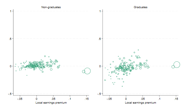
As a robustness check, I estimate an alternative two-way fixed effects model with TTWA fixed effects, as opposed to firm fixed effects. This is the traditional way of calculating local earnings premiums (Combes, Duranton and Gobillon, 2008; Gibbons, Overman and Pelkonen, 2014; De La Roca and Puga, 2017; Overman and Xu, 2024). The estimates of local earnings premiums are very similar, as shown in Figure A1 in the appendix. The correlation coefficient across the two sets of estimates is 0.88, or 0.95 weighted by population size. The main difference is that the estimated premium in London is higher when firm effects are included – likely because people who move to London often end up lower down the local firm hierarchy, and vice versa for people who leave London, which attenuates the estimates without firm effects (Card, Rothstein and Yi, 2025). Results on mobility patterns and the contribution of mobility to earnings inequalities are very similar using this alternative approach. I also estimate the model with firm fixed effects separately for graduates and for non-graduates and find very similar estimates of local earnings premiums for both groups (correlation coefficient 0.88, or 0.98 weighted by population size), consistent with previous research using TTWA fixed effects (Overman and Xu, 2024).

More details on the LEO dataset can be found in Britton et al. (2021), and details on the calculation of local earnings premium are given in Card, Rothstein and Yi (2025). The next section sets out the local earnings premiums facing young people across England, and what these tell us about the geography of opportunity.

3. Geographical differences in pay for young workers

There are large differences in pay for young workers across the country. In 2019, workers born between 1986 and 1997 were paid £18,740 a year on average in Bridlington and £19,400 a year in Penzance, in nominal terms. At the other end of the spectrum, average pay for these cohorts was £30,630 in London and £29,150 in Slough & Heathrow.

Figure 1 shows differences in real pay across the 2012–19 period, relative to the average across all TTWAs.3 In Bridlington and Penzance, young workers earned 16% and 15% less than in the average TTWA, whilst those in London and Slough & Heathrow earned 21% and 19% more. Young workers in Birmingham – England’s second-largest city – earned just 3% more than the average across all TTWAs, and pay in Manchester was no higher than in the average TTWA.

Figure 1. Raw pay differences by TTWA, 1986–97 birth cohorts in 2012–19 

_{Note: Controls for financial year effects only. Normalised to unweighted average across all TTWAs.}

Some of these differences in pay reflect who lives where. For example, only 29% of young workers living in Bridlington had an undergraduate degree at age 27, compared with 45% in London.4 Differences in average pay adjusted for individual characteristics, using the method outlined in Section 2, are shown in Figure 2. These represent the expected earnings premiums or penalties that a given young worker would face in different TTWAs.

Figure 2. Local earnings premiums by TTWA, 1986–97 birth cohorts in 2012–19 

_{Note: Estimated using method outlined in Box 1. Normalised to unweighted average across all TTWAs.}

The variation in local earnings premiums is smaller than the variation in pay levels, but still substantial. Young workers can expect to earn 15% more in London, and 14% more in Slough & Heathrow, than in the average TTWA. The place with the third-highest earnings premium is Whitehaven, a hub for the nuclear industry, which has a premium of 7%; this is the only TTWA in the top ten that is not in the South East or within commuting distance to London.5 Moreover, the ranking of places in terms of local earnings premiums is very similar to the ranking in terms of raw pay levels, with a correlation coefficient of 0.91, or 0.94 weighted by population size (see Figure A2 in the appendix).

The earnings premiums shown in Figure 2 represent the change in pay levels that one would expect when moving from one TTWA to another.6 But previous research has shown that some places offer faster pay growth as well as higher pay levels, and that spending time in high-paying cities can have lasting effects even if people eventually move out of these cities (D’Costa and Overman, 2014; De La Roca and Puga, 2017).

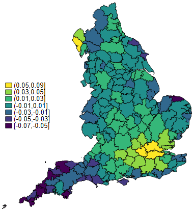
These dynamic effects are difficult to estimate robustly in the LEO data, as we do not observe the entire location histories of older cohorts, and the cohorts for whom we do have entire location histories (the 1996 birth cohort onwards) have not been in the labour market for very long.7 Nevertheless, simple comparisons suggest that high-paying places in England also offer faster pay growth, especially for graduates. Figure 3 shows that graduates who have just entered the labour market earn about 15% more in London than those in the lowest-paying fifth of TTWAs (based on their estimated earnings premiums) – £19,130 compared with £16,660 a year in 2015 prices. But eight years into their careers, that gap nearly quadruples: in London, graduates with eight years’ experience earn £42,180 on average in 2015 prices, 57% more than those in the lowest-paying TTWAs (£26,910).

Figure 3. Mean annual real earnings by years of experience and graduate status, 2015 prices

_{Note: TTWAs are grouped into quintiles based on estimated local earnings premiums. Quintile 1 denotes the lowest-paying TTWAs.}

The difference in earnings progression between London and other TTWAs in the highest-paying quintile is also striking. In the first year of their careers, there is virtually no difference in average earnings between graduates in London and those in high-paying TTWAs – a group that includes Reading, Oxford, Cambridge, Bristol and several TTWAs around London. The gap opens up over time, so that for graduates with eight years’ experience, average earnings in London are 18% higher. Outside the top quintile, earnings progression looks very similar – differences between the bottom quintile and the fourth quintile are relatively small.

Some of these gaps will reflect differences in the composition of workers across places, including selective retention – the kinds of graduates who choose to stay in London as their careers progress will differ from those who leave. But large gaps in pay progression remain after controlling for observable characteristics, as shown in Figure A3 in the appendix. Graduates who have just entered the labour market earn 16% more in London than similar graduates in the bottom fifth of TTWAs, but eight years into the labour market, this gap widens to 43%.8 Comparing graduates in London with those in other TTWAs in the highest-paying quintile, the gap widens from 5% to 17%.9

In summary, there are large geographical inequalities in labour market opportunities facing young people in England. London and surrounding areas offer much better pay prospects, in terms of both levels and opportunities for career progression, than places in Cornwall, Lincolnshire and the North. The rest of this report examines how these disparities in labour market opportunities shape patterns of geographical mobility, and how mobility patterns in turn exacerbate geographical divides.

4. Mobility between ages 16 and 27

This section examines how young people move at the start of their careers – up to age 27 – building on previous work in Britton et al. (2021). I focus on the two oldest cohorts in LEO: those who sat their GCSE exams in 2002–03 (approximately the 1986–87 birth cohorts), who were 32–33 years old in the latest pre-pandemic data. The next section will follow the same cohorts into their early 30s, looking at mobility between the ages of 27 and 32.

Young workers in England are highly mobile, as documented in Britton et al. (2021). At age 27, a fifth (21%) of the 1986–87 birth cohorts live in a different TTWA from the one in which they lived at age 16. Graduates are particularly mobile, with one in three (33%) graduates living in a different TTWA at age 27, compared with 15% of non-graduates.

High-skilled people move to high-paying cities

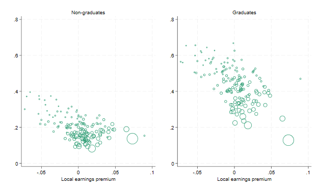
Graduate mobility is closely linked to local economic opportunity. Figure 4 plots net migration at age 27 against local earnings premiums by TTWA.10 For graduates, there is a clear positive relationship.11 By age 27, there are 46% more graduates living in London than the number of people from London, in the same cohorts, who go on to get a degree. Around half of the relationship (slope) between net migration and local opportunities is due to out-migration – graduates leaving places that offer poor opportunities – and around half to in-migration, with graduates who move choosing places that offer better opportunities (see Figures A4 and A5 in the appendix).12 In contrast, non-graduate migration does not appear to be driven by local economic opportunities.13

Figure 4. Correlation between net migration (vertical axis) and local earnings premiums (horizontal axis), ages 16–27

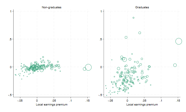
_{Note: Size of bubbles denotes total resident population of 1986–87 birth (2002–03 GCSE) cohorts at age 16. Premiums normalised to unweighted average across all TTWAs. Outliers for graduates are Brighton (0.89 net migration), Bristol (0.61) and Leeds (0.53).}

Early-career moves for graduates also tend to be towards cities. This can be seen in Figure 4, where the size of dots represents population size. At any given level of earnings premium, larger TTWAs experience higher net migration of graduates. Again, this pattern is driven by both in- and out-migration: at any given premium, larger TTWAs draw in more migrants and lose fewer residents to out-migration (Figures A4 and A5).

These flows are shown in more detail in Figure 5, which plots flows of movers between London, other major cities, smaller cities and rural areas. Cities are defined based on the Primary Urban Areas listed by the Centre for Cities,14 and the nine largest cities outside London are labelled ‘other major cities’. Graduate flows out of London are rare, and flows into London are substantial, with over a quarter (28%) of movers from outside London moving to the capital. On the other hand, 37% of all graduate movers come from rural areas, but only 19% move to rural areas.15 43% of the variation in net graduate migration across TTWAs can be explained by the local earnings premium and (log) population size.16 Unlike graduates, non-graduates are just as likely to move into rural areas as they are to leave them: the distribution of movers across area types is virtually identical at ages 16 and 27.

Figure 5. Flows of movers across area types, age 16 (left) and age 27 (right)

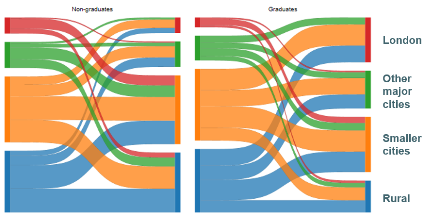
_{Note: In each panel, the left-hand side shows the distribution of movers across area types at age 16 and the right-hand side shows the distribution at age 27, with flows showing where they move from/to. Non-movers are not shown on this graph.}

Figure 6 shows that there is a clear pattern of selective mobility in early career moves – of higher-skilled workers moving to higher-paying TTWAs – going beyond the simple graduate/non-graduate distinction. The left-hand panel shows that for young people who are not from London, the probability of moving increases steeply with educational attainment. Just one in seven (14%) of those in the bottom fifth of GCSE scores live outside their TTWA of origin at 27, compared with nearly half (45%) of those in the top twentieth. In contrast, there is no relationship between educational attainment and the propensity to move for young workers from London.

Figure 6. Probability of moving (left) and share of movers moving to a higher-paying TTWA (right), by GCSE ventile, ages 16–27

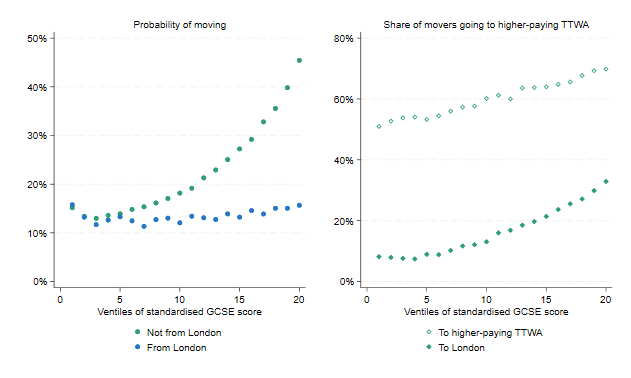
_{Note: Overall GCSE scores are standardised at the cohort level. Right-hand panel excludes those from London.}

Not only are higher-educated young people more likely to move, they are also more likely to move to places offering better economic opportunities. The right-hand panel of Figure 6 shows that for movers in the top twentieth of GCSE scores, more than two-thirds (70%) move to a TTWA with a higher local earnings premium and a third (33%) move to London. In contrast, for movers in the bottom fifth of GCSE scores, just over half (53%) of movers move to a higher-paying TTWA and only 8% move to London.

Early-career mobility brings the very highest-educated workers into London. 13% of those in the top twentieth of GCSE scores come from London – just slightly more than would be expected given London’s population share (12% in these cohorts). By age 27, the share of the highest-educated workers living in London nearly doubles to 24%.

Early-career mobility exacerbates geographical inequalities

Patterns of mobility are shaped by the geography of economic opportunity: high-skilled young people move to cities offering high pay premiums. In turn, this exacerbates geographical inequalities, by concentrating skilled workers in certain places and amplifying their individual advantages.

To quantify the effect of mobility on local earnings at age 27, I construct a simple counterfactual: what would local average earnings look like if no one moved? Using estimates from the two-way fixed effects regression (see Box 1), I first replace the firm component of each individual’s earnings with the average firm effect in their TTWA of origin. I then assign each person back to their area of origin, and calculate average (log) earnings by TTWA of origin. This yields the distribution of earnings across places in the absence of migration.

This approach abstracts from general equilibrium effects – it does not account for potential effects of the local composition of people on local earnings premiums. To the extent that we expect a higher concentration of skills to increase local premiums (if having more high-skilled people in London makes it more productive), we can think of the result as a conservative estimate of the contribution of migration to geographical earnings inequality.17

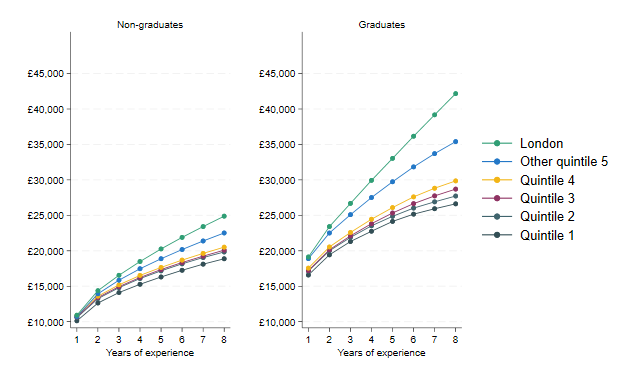
The results of this exercise are shown in Figure 7. Dark purple shades indicate a large decrease in average earnings as result of migration, and bright yellow shades indicate a large increase. London is the main beneficiary of migration between ages 16 and 27, with average earnings that are approximately 3.9% higher than in the counterfactual with no migration. Leeds is the second biggest beneficiary (3.5%), and other cities such as Reading, Bath, Bristol and Newcastle also gain, by between 1% and 2%. Coastal areas tend to lose out, with migration reducing average earnings by more than 5% in some parts of Cornwall, Yorkshire and Lincolnshire. The variance of log average earnings at age 27 – a common measure of geographical disparities – is 28% lower in the counterfactual with no mobility than it actually is (0.00486 as opposed to 0.00677). Put differently, 28% of the observed variation in earnings across TTWAs at age 27 can be attributed to mobility patterns in adulthood.

Figure 7. Estimated change in average log earnings due to migration, ages 16–27

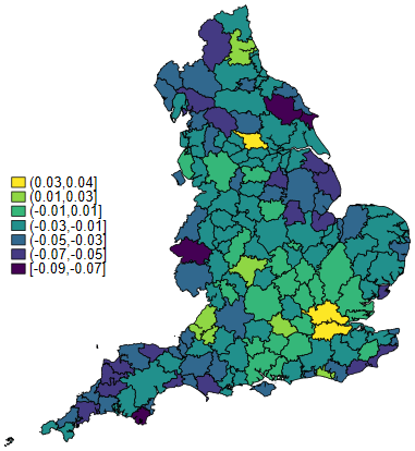
_{Note: Shows difference between actual (observed) log average earnings by TTWA and counterfactual in which no one moved. Values can be interpreted as approximately percentage differences, e.g. a gap of 0.04 means that actual earnings are approximately 4% higher than in the counterfactual with no mobility.}

5. Mobility between ages 27 and 32

The previous section showed that patterns of mobility in early careers widen geographical earnings inequalities. However, people may choose to move out of cities and return to their home towns as they get older. Indeed, net migration into London is positive only among people in their 20s; in recent years, outflows of 30- to 44-year-olds from London have exceeded inflows of 20- to 29-year-olds (Stansbury, Turner and Balls, 2023). In this section, I therefore extend the analysis in Britton et al. (2021) to examine mobility between ages 27 and 32, a stage of life when many people settle down, buy their first home and have children.18

The analysis is restricted to individuals who are employed at both 27 and 32, who make up 83% of the sample in the previous section. As Table A1 in the appendix shows, the two samples are very similar in terms of demographic characteristics, educational attainment and mobility. Those who are employed at both 27 and 32 have slightly (4%) higher earnings at age 27, but the degree of geographical earnings inequality at age 27 – as measured by the variance of log average earnings by TTWA – is nearly identical across the two groups.

Many people move in their 30s – but not in the same ways

Young people are highly mobile between ages 27 and 32, as shown in Table 1. One in five (20%) live in a different TTWA at age 32 from the one in which they lived at age 27.19 Of those who stayed in their TTWA of origin at age 27, 15% live in a different TTWA at age 32. This share is much higher for graduates: a quarter (24%) of stayers in the first period move in the second.

Table 1. Mobility trajectories aged 16–27 and aged 27–32

_{Note: (Stay, move) refers to workers who were in the same TTWA at age 27 as at age 16, but a different TTWA at age 32 from at age 27. Vice versa for (move, stay) and so on. Columns add up to 100%.}

Of those who moved to a different TTWA by age 27, 37% move again between ages 27 and 32. This share is similar for graduates and non-graduates, but non-graduates are more likely to return to their TTWA of origin (17% of movers compared with 12%), whereas graduates are more likely to move to a new TTWA (27% compared with 19% of movers). I refer to the former group as ‘returners’ and the latter group as ‘onward movers’.

Whilst the overall rate of mobility between ages 27 and 32 is similar to the rate between ages 16 and 27, patterns of mobility are very different. Graduates no longer flock to high-paying places as they did at the start of their careers (Figure 8). In particular, net graduate migration to London is close to zero in this period – just 3%, compared with 46% between ages 16 and 27.

Figure 8. Correlation between net migration (vertical axis) and local earnings premiums (horizontal axis), ages 27–32

_{Note: Size of bubbles denotes total resident population of 1986–87 birth (2002–03 GCSE) cohorts at age 27. Premiums normalised to unweighted average across all TTWAs.}

Furthermore, graduates in their late 20s and 30s do not tend to move to cities. Figure 9 shows that the distribution of graduate movers across area types is similar at ages 27 and 32. There are large inflows into London – 17% of all graduates who move go to London (20% of movers from outside London) – but these are balanced by large outflows from London, consisting of 15% of all graduate movers. Other major cities show a similar story – the next nine largest cities make up 17% of all graduate outflows and 18% of all inflows.

Figure 9. Flows of movers across area types, age 27 (left) and age 32 (right)

_{Note: In each panel, the left-hand side shows the distribution of movers across area types at age 27 and the right-hand side shows the distribution at age 32, with flows showing where they move from/to. Non-movers are not shown on this graph.}

Mobility in early 30s does not undo sorting from earlier moves

Seeing as many young people move out of cities between ages 27 and 32, with one in seven (14%) of those who moved before age 27 now returning to their TTWA of origin, one might expect migration in this later phase to undo some of the sorting that happens through earlier moves. In fact, this is not the case: migration between ages 27 and 32 further increases geographical inequalities.

There are three key reasons for this. First, many high-skilled people move for the first time after age 27, and move in similar ways to high-skilled people at earlier ages. Among this group, high-skilled workers are more likely to move to high-paying TTWAs, exacerbating geographical inequalities. Second, return migration is ‘negatively selected’, with low-skilled people being more likely to return to their TTWA of origin. Third, whilst many of those who move to London at the start of their careers leave the capital by age 32, they mostly move to other prosperous areas in the South East. I consider each of these factors in turn.

Many high-skilled people move for the first time after age 27

As set out above, a quarter (24%) of graduates who lived in their TTWA of origin at age 27 live in a different TTWA at age 32. This implies that many high-skilled people move for the first time between ages 27 and 32.20 Figure 10, which plots the distribution of GCSE scores across different groups of movers, shows that these ‘first-time movers’ (the blue line) are similar in terms of educational attainment to those who move by age 27 (the yellow line).

Figure 10. Distribution of GCSE scores by mobility trajectory

_{Note: Shows Epanechnikov kernel density plot. Overall GCSE scores are standardised at the cohort level.}

These first-time movers also move in similar ways to earlier movers, with higher-educated workers moving to higher-paying TTWAs. This is shown in Figure 11, where the left panel shows movers between 16 and 27 (equivalent to the right-hand panel of Figure 621) and the right panel shows people moving for the first time after age 27. Patterns across the two groups are very similar. Among the latter group, 63% of those in the top GCSE ventile move to a TTWA with a higher local earnings premium and 28% move to London. For those in the bottom ventile, the figures are 40% and 4% respectively.

Figure 11. Share of movers moving to a higher-paying TTWA by GCSE ventile, ages 16–27 (left) and ages 27–32 (right)

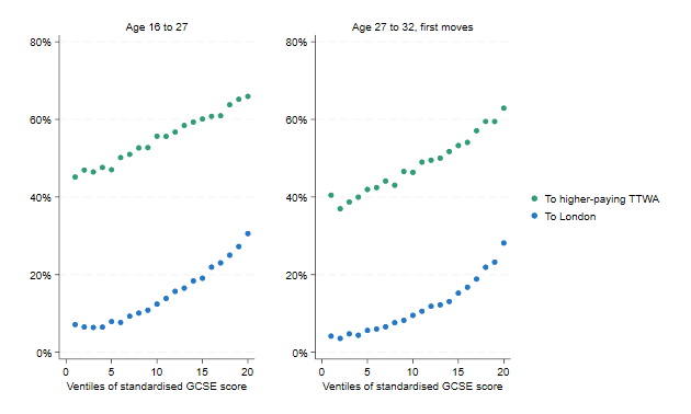
_{Note: Overall GCSE scores are standardised at the cohort level.}

In other words, many people are moving for the first time between ages 27 and 32, and they look like earlier movers and move in similar ways, continuing earlier patterns of sorting.

Return migration is negatively selected

Of those who move by age 27, one in seven (14%) return to their TTWA of origin by age 32. One might expect this to undo some of the sorting from earlier moves. In practice, however, this does not have a big effect, as returners are more likely to be low-skilled.

Table 1 above shows that return migration is more common among non-graduates: more than one in six (17%) non-graduate movers return to their TTWA of origin by age 32, compared with fewer than one in eight (12%) graduate movers. Figure 12, which goes beyond the graduate/non-graduate distinction, shows that GCSE attainment is lower among returners than among migrants who do not return (though still higher than those who do not move by age 27).

Figure 12. Distribution of GCSE scores by mobility trajectory

_{Note: Shows Epanechnikov kernel density plot. Overall GCSE scores are standardised at the cohort level.}

Furthermore, return migration is more common among those from higher-paying areas, as shown in Figure 13. This is especially true for graduates. 18% of graduates from London who leave by age 27 return to London by age 32. Looking across the top 10 TTWAs in terms of local earnings premiums (including London), 14% of graduate migrants return by age 32. In contrast, of graduates who move out of the lowest-paying 10 TTWAs in their early careers, only 9% return.

Figure 13. Correlation between probability of return migration (vertical axis) and local earnings premiums in TTWA of origin (horizontal axis)

_{Note: Horizontal axis shows local earnings premiums of age-16 TTWA. Premiums normalised to unweighted average across all TTWAs.}

Movers from London go to prosperous areas in the South East

Finally, although many workers who moved to London by age 27 leave the capital by age 32, they tend to move to already-prosperous areas in the South East, not to low-paid parts of the country.

One in five (19%) young workers living in London at age 27 move elsewhere by age 32, including one in three (34%) of those who are not originally from London. Of the latter group, the majority (62%) move to a TTWA that is not their TTWA of origin. These ‘onward movers’ are very highly educated, both compared with other movers and with London residents – 77% have an undergraduate degree (Table 2). Half (48%) of onward movers from London move to TTWAs that border London. These are places that already have high levels of pay: on average, young workers can expect to earn 6% more in these TTWAs than in the average TTWA.22

Table 2. Educational attainment by move trajectory

_{Note: Sample sizes rounded to nearest 10. ‘Onward movers’ refers to those who move between ages 16 and 27, and again between ages 27 and 32, but do not return to their TTWA of origin.}

Figure 14 maps the number of movers to London between ages 16 and 27 (left) and the number of return and onward movers from London between ages 27 and 32 (right), by TTWA as a percentage of all residents at the start of the period. In both cases, figures are scaled by the total number of movers (to and from London respectively) as a percentage of the total population, which allows both maps to be shown on the same scale. A value of 1 implies that a TTWA has as many movers to (left) as from (right) London, as you would expect if movers were randomly distributed.

Figure 14. Origins of movers to London aged 16–27 and destinations of return and onward movers from London aged 27–32

_{Note: Shows number of migrants to (from) London in a TTWA as a share of the population of that TTWA at the start of the period, scaled by the total number of migrants as a share of the total population.}

A striking feature of Figure 14 is that moves from London are much more spatially concentrated than moves to London at the start of people’s careers. In this way, London redistributes talent from the rest of the country to the South East. Skilled workers from all over the country move to London at the start of their careers, and subsequently move to TTWAs just outside London. This is not true of other cities – for example Manchester, which mainly draws early-career workers from neighbouring TTWAs and moves them back out to neighbouring TTWAs in their early 30s (Figure 15).

Figure 15. Origins of movers to Manchester aged 16–27 and destinations of return and onward movers from Manchester aged 27–32

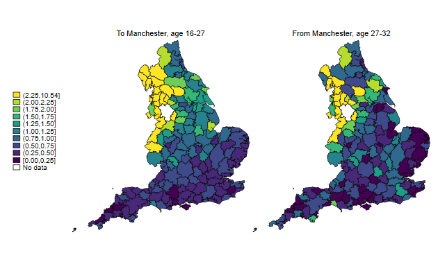
_{Note: Shows number of migrants to (from) Manchester in a TTWA as a share of the population of that TTWA at the start of the period, scaled by the total number of migrants as a share of the total population.}

It is worth noting that the maps in Figures 14 and 15 show workers by place of residence, not place of work. Two-thirds (66%) of workers who move from London to a neighbouring TTWA between ages 27 and 32 stay at the same enterprise in the year of the move. It is likely that many remain in the same workplace and commute to London (as noted in Section 2, the LEO data do not contain information on local units, so we cannot tell whether people are commuting to the same workplace or moving to another branch of the same enterprise). As such, benefits to TTWAs bordering London may not accrue to firms in these places, though providers of local services will benefit from higher spending power.

Nearly 40% of geographical earnings inequality at age 32 is due to migration

Patterns of migration between ages 27 and 32 further exacerbate geographical inequalities in earnings. As stated in Section 4, 13% of young workers in the top 5% of GCSE scores are from London, but 24% live in London by age 27. At age 32, the share is higher still at 26%. A further 14% live in TTWAs that border London, so that London and surrounding TTWAs make up 40% of the very highest-educated workers. Of workers in the top 5% of GCSE scores who are not from London, 59% live outside their TTWA of origin at age 32, 30% of whom live in London.

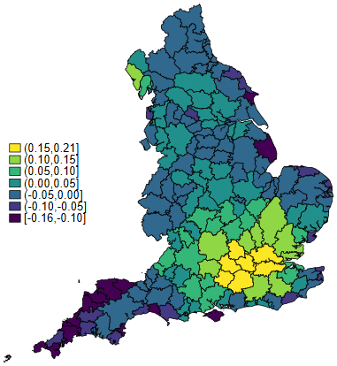
The right-hand panel of Figure 16 shows the difference in average log earnings at age 32 in each TTWA, relative to a counterfactual in which no one left their TTWA of origin, repeating the exercise described in the previous section. The left-hand panel is equivalent to Figure 7, showing the difference at age 27.23

Figure 16. Estimated change in log average earnings due to migration, ages 16–27 (left) and ages 27–32 (right)

_{Note: Shows difference between actual (observed) log average earnings by TTWA and counterfactual in which no one moved. Values can be interpreted as approximately percentage differences, e.g. a gap of 0.04 means that actual earnings are approximately 4% higher than in the counterfactual with no mobility. Sample is people in employment at both age 27 and age 32.}

Comparing the two panels, we see that mobility patterns between ages 27 and 32 further widen geographical earnings inequalities. Coastal areas that lose talent early on (shown in dark purple) lose even more by age 32, whilst areas that gain from early-career mobility (shown in green/yellow) pull further ahead. Average earnings in London at age 32 are approximately 8% higher than in the counterfactual with no migration, whilst parts of Cornwall, Yorkshire and Lincolnshire have average earnings that are 7% lower. Of the 15 TTWAs outside London that benefit from migration (have higher earnings than in the counterfactual with no migration), five border London. Bath, Brighton, Bristol, Leeds and Oxford also gain by between 2% and 4%.

The overall level of geographical earnings inequality at age 32 – measured by the variance of average log earnings by TTWA – is 39% lower in the counterfactual with no mobility than it actually is (0.00687 as opposed to 0.01125). Put differently, 39% of the observed variation in earnings across TTWAs at age 32 can be attributed to mobility.

6. Changes in mobility across cohorts

The previous sections focus on the cohorts born in 1986 and 1987, who were 32–33 years old in the latest pre-pandemic data. This section considers whether rates and patterns of mobility changed in more recent cohorts.

Figure 17 shows the share of workers living outside their TTWA of origin by age and birth cohort, with the oldest cohorts in dark purple and the youngest in bright yellow. It shows that in every cohort, mobility increases with age, with a steepening of the slope at age 21 when graduates (who are more mobile) enter the labour market. What is striking is that at every age, younger cohorts are consistently more mobile than older ones. For example, at age 27, a quarter (25%) of those born in 1992 lived in another TTWA, compared with a fifth (21%) of those born in 1986.

Figure 17. Share living in different TTWA from origin (age 16) TTWA, by age and birth cohort

_{Note: 1986 birth cohort refers to the 2002 GCSE cohort, most of whom were born between September 1985 and August 1986. Age is inferred from GCSE cohort and financial year, rather than calculated from dates of birth.}

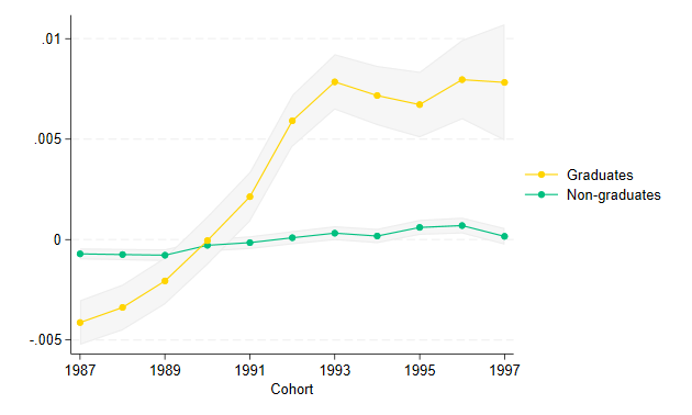
Differences in mobility by cohort could reflect differences in the composition of cohorts. For example, higher education participation has increased over time, and graduates are more mobile. To account for this and other observable differences across cohorts, Figure 18 shows the probability of living outside one’s TTWA of origin, relative to the 1986 cohort, holding constant individual characteristics (including TTWA of origin and single year of age). The analysis is conducted separately for graduates and non-graduates.

Figure 18. Probability of living outside TTWA of origin relative to 1986 birth cohort, controlling for observables

_{Note: Shows estimated cohort effects from a linear probability model controlling for TTWA of origin, single year of age, gender, ethnic group, free school meals (FSM) and special educational needs (SEN) status at age 16, whether English is an additional language (EAL) and within-cohort standardised English and mathematics scores at Key Stage 4. Regression for graduates also controls for university-and-subject groups.}

Even adjusting for individual characteristics, the trend is clear: young workers – especially graduates – have become more mobile over time. Graduates born in 1996 are 8 percentage points more likely to live outside their TTWA of origin than those born in the 1986 cohort, all else equal. For non-graduates, the difference is 5 percentage points. Furthermore, the increase in mobility has – until very recently for graduates – been steeper among young workers from low-paying TTWAs, as shown in Figure 19.

Figure 19. Probability of living outside TTWA of origin relative to 1986 birth cohort, controlling for observables, by local earnings premium in TTWA of origin

_{Note: Shows estimated cohort effects from a linear probability model controlling for TTWA of origin, single year of age, gender, ethnic group, free school meals (FSM) and special educational needs (SEN) status at age 16, whether English is an additional language (EAL) and within-cohort standardised English and mathematics scores at Key Stage 4. Regression for graduates also controls for university-and-subject groups. Cohort effects are interacted with a dummy for being from a TTWA in the lowest three quintiles of local earnings premiums.}

More recent cohorts are also more likely to move to higher-paying TTWAs, conditional on observed characteristics – unsurprisingly as mobility has increased more for workers from low-paying places. Figure A6 in the appendix shows that relative to the 1986 cohort, graduates born in 1996 are 5 percentage points more likely to move to a TTWA with a higher local earnings premium than their TTWA of origin, whilst non-graduates are 2 percentage points more likely to do so.24

The probability of moving to London has also increased very slightly in recent cohorts. After dipping for the 1987–89 cohorts, who entered the labour market during the financial crisis, the probability of moving to London recovers and stabilises around the 1993 cohort. Among graduates born after 1993, the share moving to London is just under 1 percentage point higher than for those born in 1986, all else equal (see Figure A7).

7. Conclusion

Economic opportunities facing young people vary widely across the country. Many people do not move, which means that their career prospects will be constrained by the opportunities where they grow up. But many people – especially graduates – do move, and their mobility patterns in turn shape the distribution of economic performance across places.

This report shows that high-skilled workers move to cities offering better opportunities at the start of their careers, which widens geographical inequalities in pay. Mobility remains high in people’s 30s, though patterns shift. However, migration in this later stage of life does not undo the sorting that results from earlier mobility, and in fact exacerbates geographical inequalities. This is because many graduates are moving for the first time; low-skilled movers are more likely to return to their home towns; and those who move on from London mostly move to already-prosperous areas in the South East. By age 32, nearly 40% of the variation in average earnings across places can be explained by mobility.

Despite the focus on reducing geographical disparities (‘levelling up’) in recent years, younger cohorts have become increasingly mobile over time, and more likely to move to places with better economic prospects. This suggests that migration could be playing an increasing role in widening geographical inequalities.

The importance of mobility means that policies to raise educational attainment in deprived places are unlikely to boost local economic performance on their own. Without local opportunities – good jobs that are well matched to workers’ skills, and productive firms providing those good jobs and training and development pathways – high-skilled people will continue to leave for places offering better prospects. Those who are not able or willing to move will not be able to make full use of their skills. Reducing economic disparities between places therefore requires bringing opportunity to people – not just raising skills, but building places where skills are rewarded.

Appendix

Figure A1. Correlation between local earnings premiums estimated at the firm level (vertical axis) and at the TTWA level (horizontal axis)

_{Note: Size of bubbles denotes total resident population of 1986–87 birth (2002–03 GCSE) cohorts at age 16. Premiums normalised to unweighted average across all TTWAs.}

Figure A2. Correlation between TTWA-level earnings differences with (vertical axis) and without (horizontal axis) controlling for differences in individual characteristics

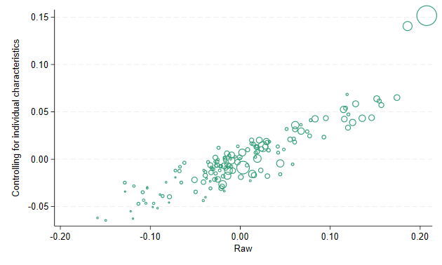
_{Note: Size of bubbles denotes total resident population of 1986–87 birth (2002–03 GCSE) cohorts at age 16. ‘Raw’ premiums based on regression that controls only for financial year effects. Premiums normalised to unweighted average across all TTWAs.}

Figure A3. Differences in log earnings compared with lowest-paying quintile of TTWAs, controlling for observable characteristics, by graduate status and years of experience

_{Note: Based on regression of log earnings controlling for gender, ethnic group, free school meals (FSM) and special educational needs (SEN) status at age 16, whether English is an additional language (EAL) and within-cohort standardised English, mathematics and overall scores at Key Stage 4, estimated separately by graduate status and years of experience. Regression for graduates also controls for university-and-subject groups.}

Figure A4. Correlation between out-migration (vertical axis) and local earnings premiums (horizontal axis), ages 16–27

_{Note: Size of bubbles denotes total resident population of 1986–87 birth (2002–03 GCSE) cohorts at age 16. Premiums normalised to unweighted average across all TTWAs.}

Figure A5. Correlation between in-migration (vertical axis) and local earnings premiums (horizontal axis), ages 16–27

_{Note: Size of bubbles denotes total resident population of 1986–87 birth (2002–03 GCSE) cohorts at age 16. Premiums normalised to unweighted average across all TTWAs.}

Table A1. Sample characteristics

_{Note: Shows characteristics for individuals in 1986–87 birth (2002–03 GCSE) cohorts who were employed at age 27 and for individuals who were employed at both age 27 and age 32.}

Figure A6. Probability of moving to higher-paying TTWA relative to 1986 birth cohort, controlling for observables

_{Note: Shows estimated cohort effects from a linear probability model controlling for TTWA of origin, single year of age, gender, ethnic group, free school meals (FSM) and special educational needs (SEN) status at age 16, whether English is an additional language (EAL) and within-cohort standardised English and mathematics scores at Key Stage 4. Regression for graduates also controls for university-and-subject groups.}

Figure A7. Probability of moving to London relative to 1986 birth cohort, controlling for observables

_{Note: Shows estimated cohort effects from a linear probability model controlling for TTWA of origin, single year of age, gender, ethnic group, free school meals (FSM) and special educational needs (SEN) status at age 16, whether English is an additional language (EAL) and within-cohort standardised English and mathematics scores at Key Stage 4. Regression for graduates also controls for university-and-subject groups.} 

References

Abowd, J. M., Kramarz, F. and Margolis, D.N., 1999. High wage workers and high wage firms. Econometrica, 67(2), 251–333, https://doi.org/10.1111/1468-0262.00020.

Britton, J., van der Erve, L., Waltmann, B. and Xu, X., 2021. London calling? Higher education, geographical mobility and early-career earnings. IFS Report, https://ifs.org.uk/publications/london-calling-higher-education-geographical-mobility-and-early-career-earnings.

Card, D., Rothstein, J. and Yi, M., 2025. Location, location, location. American Economic Journal: Applied Economics, 17(1), 297–336, https://doi.org//10.1257/app.20220427.

Combes, P-P., Duranton, G. and Gobillon, L., 2008. Spatial wage disparities: sorting matters! Journal of Urban Economics, 63(2), 723–42, https://doi.org/10.1016/j.jue.2007.04.004.

Cribb, J., 2019. Intergenerational differences in income and wealth: evidence from Britain. Fiscal Studies, 40(3), 275–99, https://doi.org/10.1111/1475-5890.12202.

D’Costa, S. and Overman, H. G., 2014. The urban wage growth premium: sorting or learning? Regional Science and Urban Economics, 48, 168–79, https://doi.org/10.1016/j.regsciurbeco.2014.06.006.

De La Roca, J. and Puga, D., 2017. Learning by working in big cities. Review of Economic Studies, 84(1), 106–42, https://doi.org/10.1093/restud/rdw031.

Engbom, N., Moser, C. and Sauermann, J., 2023. Firm pay dynamics. Journal of Econometrics, 233(2), 396–423, https://doi.org/10.1016/j.jeconom.2022.01.012.

Gibbons, S., Overman, H. G. and Pelkonen, P., 2014. Area disparities in Britain: understanding the contribution of people vs. place through variance decompositions. Oxford Bulletin of Economics and Statistics, 76(5), 745–63, https://doi.org/10.1111/obes.12043.

Lachowska, M., Mas, A., Saggio, R. and Woodbury, S., 2023. Do firm effects drift? Evidence from Washington administrative data. Journal of Econometrics, 233(2), 375–95, https://doi.org/10.1016/j.jeconom.2021.12.014.

Overman, H. G. and Xu, X., 2024. Spatial disparities across labour markets. Oxford Open Economics, 3(Supplement 1), i585–610, https://doi.org/10.1093/ooec/odae005.

Stansbury, A., Turner, D. and Balls, E., 2023. Tackling the UK’s regional economic inequality: binding constraints and avenues for policy intervention. Contemporary Social Science, 18(3–4), 318–56, https://doi.org/10.1080/21582041.2023.2250745.

Data

Department for Education; HM Revenue and Customs; Department for Work and Pensions; Higher Education Statistics Agency, released 01 November 2023, ONS SRS Metadata Catalogue, dataset, Longitudinal Education Outcomes SRS Iteration 2 Standard Extract - England, https://doi.org/10.57906/pzfv-d195.

University of Essex, Institute for Social and Economic Research. (2024). Understanding Society: Waves 1-14, 2009-2023 and Harmonised BHPS: Waves 1-18, 1991-2009. [data collection]. 19th Edition. UK Data Service. SN: 6614, http://doi.org/10.5255/UKDA-SN-6614-20.

Acknowledgements

This work was supported by ADR UK (Administrative Data Research UK), an Economic and Social Research Council (ESRC) investment (part of UK Research and Innovation) [grant number: ES/Y001249/1]. The author gratefully acknowledges the support of the ESRC Centre for the Microeconomic Analysis of Public Policy (ES/T014334/1). This work was undertaken in the Office for National Statistics (ONS) Secure Research Service using data from ONS and other owners and does not imply the endorsement of the ONS or other data owners.