Public finances: where are we now?

4.1 Introduction

Since the financial crisis, public sector borrowing – the gap between government revenue and spending – has fallen rapidly and, at the March 2019 Spring Statement, it stood below its long-run historical average. However, a number of changes have occurred since March or loom on the horizon. The new accounting treatment of student loans dispels a ‘fiscal illusion’ that was previously flattering headline measures of borrowing. The September 2019 Spending Round has, according to the government, ‘turned the page on austerity’. The most recent Bank of England growth forecasts warned of the chances of an imminent recession. Finally, the Brexit process (perhaps) risks delivering a significant adverse shock to the public finances via a non-negotiated exit from the EU.

In Section 4.2, we contextualise the current situation of the public finances with respect to the recent past and international experience. Then in Section 4.3, we discuss changes since the Office for Budget Responsibility’s (OBR’s) last forecast for debt and borrowing at the Spring Statement in March that are already known to affect the public finances, and we produce an updated baseline forecast. In Section 4.4, we look ahead to analyse a variety of scenarios for the medium term, discussing the impact of a near-term downgrade in the growth outlook even with a smooth Brexit; a no-deal Brexit; and a potential further permanent fiscal loosening – for example, to implement cuts to income tax that were a part of the prime minister’s platform during the Conservative leadership contest.

4.2 Where are we and how did we get here?

Government receipts, spending and borrowing

The path of government receipts and spending since 1997–98, measured as a share of national income, is shown in Figure 4.1.

Government spending increased slowly as a fraction of national income during the early 2000s, rose sharply as national income fell in the wake of the financial crisis, and has since fallen considerably over the last decade. In the most recent financial year, 2018–19, both total public spending (known as total managed expenditure, TME) and day-to-day or current expenditure (TME excluding public sector net investment) were at their lowest share of national income since 2006–07.

Figure 4.1. Public sector receipts and spending since 1997–98

_{Note: Current expenditure includes depreciation. Figures are accurate as of the 24 September 2019 public finances data release.}

_{Source: Office for Budget Responsibility, ‘Public finances databank’, 30 September 2019, https://obr.uk/data/.}

The path for current government receipts, which include both tax and non-tax receipts of government (the latter includes items such as interest income), has been much more stable. But receipts have edged up over the period since 1997–98, in part due to discretionary net tax-raising measures being announced and implemented in the year or two following the 1997, 2001, 2010 and 2015 general elections. In 2018–19, they had climbed to 38.0% of national income, which had not been exceeded since 1985–86. Looking just at tax (i.e. ignoring non-tax receipts), at 34.4%, revenues are at their highest sustained level as a fraction of national income since the early 1950s.

The gap between total spending and receipts is the deficit – more formally known as public sector net borrowing. As can be seen in Figure 4.1, while the UK has not run an overall budget surplus (i.e. had current receipts that exceed TME) since 2000–01, public sector net borrowing is now lower than it was in the years prior to the financial crisis. In addition, in 2018–19, the government ran a surplus on its current budget as receipts exceeded current spending – the first time in 17 years that the UK government was not borrowing to finance day-to-day spending.

These patterns are shown more clearly in Figure 4.2, which shows overall borrowing (the extent to which total spending exceeds receipts) and the current budget deficit (the extent to which current spending exceeds receipts), again since 1997–98. In 2018–19, both were at a lower level than in any year since 2001–02.

As Figures 4.1 and 4.2 have shown, public sector net borrowing has now been brought down to less than 2%, below pre-crisis levels, through a combination of current receipts rising to their highest share of national income since 1985–86 and total public spending being reduced to its lowest share of national income since 2006–07. Borrowing is also now typical by longer-run UK historical standards: borrowing of 1.9% of national income in 2018–19 is equal to the average rate of public sector net borrowing over the 60 years from 1948 to 2007–08.

Figure 4.2. Public sector borrowing since 1997–98

_{Source: Office for Budget Responsibility, ‘Public finances databank’, 30 September 2019, https://obr.uk/data/.}

Public sector net debt and debt interest

The high levels of public sector net borrowing over the period from 2008–09 to 2015–16 (inclusive) have increased the stock of government debt substantially. Prior to the financial crisis and associated recession, public sector net debt was running at just below 40% of national income but – as shown in Figure 4.3 – it has since more than doubled as a share of national income, reaching a peak of 84% in 2016–17. This is the highest level of public sector net debt since 1963–64 (although prior to this, net debt had been continuously above this share of national income since 1915–16). Public sector net debt has since fallen as a share of national income. This is because government borrowing since 2016–17 has been sufficiently low that the cash stock of debt has grown less quickly than the cash size of the economy.

Despite this doubling of net debt, the government’s debt interest bill has remained flat in real terms as the recorded cost of government borrowing has fallen. As shown in Figure 4.3, in 2018–19, when public sector net debt exceeded 80% of national income, spending on debt interest was 1.8% of national income, or £37.5 billion in nominal terms. Compare this with 2007–08, when public sector net debt was below 40% of national income but spending on debt interest was actually higher as a share of national income, at 2.0%. A simple ‘effective annual interest rate’, calculated as annual spending on debt interest as a share of public sector net debt at the end of the preceding financial year, has fallen from around 6% just before the financial crisis to just above 2% in 2018–19. Mostly, the low debt interest cost is due to low rates on gilts (government bonds), which reflect a genuinely low cost of borrowing and can be used to justify greater borrowing. However, spending on debt interest is also currently flattered by the Bank of England’s programme of quantitative easing. If the gilts purchased under this scheme had instead been held by the private sector, debt interest spending would have been scored at around £3 billion higher in 2018–19.1

Figure 4.3. Public sector debt and debt interest since 1997–98

_{Source: Office for Budget Responsibility, ‘Public finances databank’, 30 September 2019, https://obr.uk/data/. Debt interest is net of the Bank of England’s Asset Purchase Facility (see https://www.bankofengland.co.uk/markets/quantitative-easing-and-the-asset-purchase-facility and footnote 1 at the bottom of the next page).}

International comparisons

Compared with other industrialised countries, both the UK’s deficit and its debt are above average. Figure 4.4 shows that among 25 other large economies, only seven have a higher deficit and only eight have a larger stock of debt, relative to the size of their economies. Among the countries with the highest debt stock are those hardest hit by the financial crisis, including Greece, Italy, Portugal and Spain.

Figure 4.4. Deficit and debt in 26 countries in 2018 

_{Note: Bubbles represent the size of a country’s economy in 2018 (in dollars). Debt in Czech Republic refers to 2017, not 2018; net debt not available for Greece and China so gross figure used. Measures are general government net deficit and general government net debt. These are similar to, but differ slightly from, the public sector measures typically used in the UK and quoted elsewhere in the chapter.}

_{Source: International Monetary Fund, World Economic Outlook Database, April 2019, https://www.imf.org/external/pubs/ft/weo/2019/01/weodata/index.aspx.}

The size of the dots in Figure 4.4 indicates the size of each economy. As a general rule, larger economies tend to run higher deficits and accumulate more debt as a share of national income than smaller ones, with the United States having the largest deficit and Japan both the second-largest deficit and the second-largest debt. Italy, France and the UK are also all large economies where the government deficit and debt are comparatively high relative to the size of the economy. Notable exceptions to this rule are Germany and China: both have a below-average level of debt and are running a budget surplus. Sizeable budget surpluses are also seen in South Korea and Norway (whose oil reserves are being used to accumulate substantial net assets).

4.3 Changes since the Spring Statement

On 24 September 2019, the Office for National Statistics (ONS) released its latest public finances figures. These differ considerably from the estimates of borrowing that had been released alongside the March 2019 Spring Statement, for reasons both expected and unanticipated. This section discusses the drivers behind these revisions and assesses their possible impact on the outlook for the public finances going forwards.

Student loan accounting

One of the biggest revisions to the March 2019 figures on the public finances has come from changes to the accounting methods used by the ONS, which came into effect in September 2019. The most significant of these is an important change to the way in which student loans are accounted for in the public finances. A substantial portion of student loans extended (estimated by IFS researchers to be 45% of the total outlay for those beginning to receive loans in Autumn 20192) is not expected to be repaid. Under the new methodology, the expected government loss is recorded as an increase in government borrowing at the moment the loan is extended (when the student is at university) rather than when the loan is actually written off (30 years after graduation). More details on this accounting change are given in Box 4.1.

As the new accounting treatment more accurately reflects the economic reality, the change is a welcome one. The impact on measured fiscal aggregates is to push up capital spending (and therefore total spending) and to depress current receipts. Therefore, it pushes up measures of both overall public sector net borrowing and (to a lesser extent) the current budget deficit. But, as ever, the choice of accounting methodology (and changes to it) does not directly affect the true underlying health of the public finances.

In contrast to the deficit, measures of public sector net debt are unaffected by the accounting change: all spending on student loans continues to add to debt when the loans are made, while repayments of student loans (or receipts from selling the student loan book) reduce debt in the year the funds are received.

In total, the student loan change adds £12.4 billion to borrowing in 2018–19, which accounts for the lion’s share of the upwards revision from 1.1% to 1.9% of national income since March. This amount will rise over time as more students receive loans to cover the higher fees in place since 2012. As shown in Table 4.1 (under adjustment A), our calculations suggest that it will rise to £16.1 billion in nominal terms in 2023–24.

Table 4.1. The March 2019 borrowing forecast updated for subsequent developments

_{Note: All £ billion figures in nominal terms. (A) is constructed from ONS September 2019 public finance release and OBR forecast. (B) assumes that the combined impact of changes remains roughly at the same level it has been for the past four years, as reported in the August public finance release. (C) is the direct increase in TME announced in the September 2019 Spending Round. (D) uses OBR multipliers to calculate the boost to revenues that arises as a result of the additional spending announced in the Spending Round. (E) assumes EU contributions and receipts during the transition period are the same as during membership. (F) assumes counterfactual EU spending in the UK remains constant as a share of the gross contribution, with counterfactual contributions to the EU taken from the March 2019 Economic and Fiscal Outlook.}

Corporation tax receipts and pensions

Receipts had been artificially high for several years due to an accounting error at HMRC that double-counted corporation tax credits. Correcting this error added £2.6 billion to borrowing in 2018–19. In addition, methodology and data changes related to the treatment of pensions in public sector statistics increased recorded borrowing by £1.3 billion in the same year. Figure 4.1, and all other numbers on the past state of the public finances in this chapter, are based on the updated figures for all years, released in September. For our projections, we assume that the impact of these changes on borrowing stabilises at £4 billion a year (adjustment B).

The 2019 Spending Round

On 4 September 2019, Chancellor Sajid Javid announced a substantial boost to day-to-day departmental spending. This increased planned spending in 2020–21 by £13.4 billion. In addition, he announced a three-year settlement for spending on schools in England which, if delivered, would reverse most of the cuts to day-to-day per-pupil spending seen since 2009.

Limits for day-to-day departmental spending have not been set beyond 2020–21. We assume that overall day-to-day department spending is increased in real terms so that it can cover the multi-year settlements announced for the NHS and schools in England.3 Keeping to even these increased spending limits would still mean that any other additional spending commitments – for example, to increase police numbers further and to keep defence spending and official development assistance spending at 2.0% and 0.7% of national income respectively – and any Barnett implications from the NHS and schools spending increases in England would require cuts to be found elsewhere.

As shown in Table 4.1 (adjustment C) relative to the March 2019 Spring Statement, this adds £13.4 billion to spending in 2020–21, rising to £18.5 billion in nominal terms in 2023–24.

Other adjustments

We make two other adjustments to the forecasts set out in the March 2019 Budget.

First, we allow the spending round boost to spending to increase demand in the economy, using the multipliers that the OBR applies. This increase in economic activity boosts revenues temporarily (thereby reducing the deficit), but this effect is assumed to fade over time as monetary policy, exchange rates, wages and other prices in the economy adjust (adjustment D in Table 4.1).

Second, the OBR’s forecast assumes that the UK chooses to spend the money it no longer pays the EU on unspecified domestic priorities. There is a direct saving to the public finances because the UK’s payments to the EU under the financial settlement (‘the divorce bill’) are typically lower than what the payments would have been, had the UK remained in the EU. In the March 2019 Spring Statement, the OBR assumed this saving would be spent rather than used to reduce borrowing. One could argue that the September 2019 Spending Round announcement was Mr Javid choosing to devote these funds to UK public services, but we separately account for this spending, as discussed. In line with the UK government’s commitment, we assume it replaces EU spending in the UK – for example, on farm subsidies and research funding. We then assume that any savings from EU contributions over and above this level are available to reduce borrowing or, in one of our scenarios, partly to fund an additional giveaway.

As shown in Table 4.1, the overall impact of these changes is zero in this financial year and very modest in 2020–21 because during the transition period (which is assumed to run until the end of 2020), both UK contributions to the EU and EU spending in the UK continue unchanged.4 But the saving rises to £1.5 billion in 2023–24 (as shown by the net effect of adjustments E and F). This corresponds to less than £30 million per week. This direct saving is only a small part of the impact Brexit will have on the public finances: the impact that it has had and may still have on growth, which is discussed in detail in the next section and in Chapter 3, dwarfs the direct benefits of avoiding EU contributions.

Overall change to the outlook for borrowing

Overall, the net effect of these changes is to push up headline borrowing by £21.3 billion in 2019–20. Borrowing in 2023–24 is now expected to be nearly £50 billion, £36 billion more than forecast by the OBR in March. Most of this change is explained by the (welcome) change in student loan accounting and the chancellor’s spending round decision to boost overall day-to-day spending on public services. This revised forecast for borrowing – £50.6 billion or 2.3% of national income in 2019–20, falling to 1.9% of national income in 2023–24 – implies that, on the new accounting basis, the deficit would not decrease from its 2018–19 level (1.9% of national income) over the next five years.

This adjusted borrowing forecast is essentially what we might have expected the OBR to have produced alongside the March 2019 Spring Statement had the methodological changes to the public sector statistics already come into effect, had the error in recording corporation tax receipts already been corrected and had Mr Hammond announced the additional spending for departments in 2020–21 at that point (and had the OBR changed its assumption that any direct saving from EU contributions would be spent rather than saved). There have, of course, been other developments since March. The possible impact of these on the public finances is considered in the next section.

4.4 Looking ahead

The adjustments discussed so far relate to accounting changes and firm spending commitments, which we know will affect borrowing no matter what happens to the economy. But, clearly, the outlook for the public finances depends crucially on whether, as a number of forecasters have predicted (at least for the near term), economic growth is weaker than forecast at the time of the Spring Statement, and on whether the UK leaves the EU without a deal, with the disruption to the economy that this would entail.

This section first shows how the adjusted baseline forecast might be expected to change if the OBR decided to downgrade its forecasts for growth to be in line with the Bank of England’s forecast made in August 2019 (which, like the OBR’s forecast, is predicated on a smooth Brexit). It then considers the impact of an additional permanent fiscal giveaway – on top of the spending round announcement – of 1% of national income. This is done first for scenarios in which we retain the OBR’s assumption of a ‘smooth and orderly’ Brexit process and then repeated under a – still reasonably orderly – ‘no deal’ scenario.

Smooth and orderly Brexit scenarios

The top panel of Table 4.2 simply repeats the adjusted baseline forecast for borrowing that was shown in Table 4.1, and the related forecasts for public sector net debt (excluding the Bank of England; see Box 4.2). The table also shows the forecast path for economic growth under this scenario, which is the OBR’s March 2019 growth forecasts updated to take into account the temporary boost to economic activity that might be expected from the spending round announcement.

Table 4.2. Scenarios for the public finances in a smooth-Brexit scenario

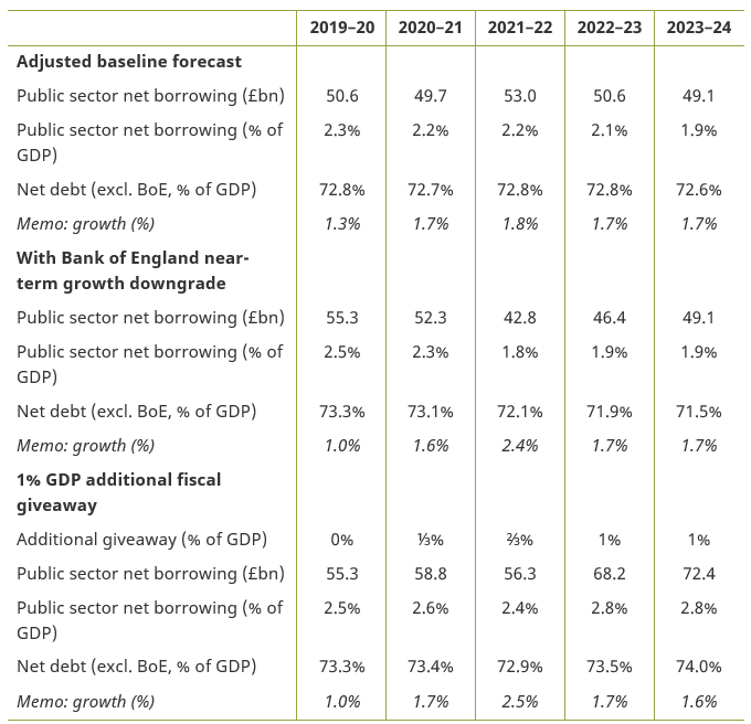
_{Note: The adjusted baseline forecast is as shown in Table 4.1. ‘Bank of England’ growth forecast additionally updates for the August 2019 Bank forecast. Additional 1% giveaway is permanent and phased in over three years, starting in 2020–21. Debt excluding Bank of England (BoE) assumes that the Bank’s contribution to debt is unaffected by the scenarios considered.}

_{Source: Office for Budget Responsibility, Economic and Fiscal Outlook: March 2019; Bank of England, Inflation Report: August 2019.}

Box 4.1. Headline debt figures and the Term Funding Scheme

The OBR’s March 2019 Spring Statement forecasts were for public sector net debt to continue falling over the coming years (see Figure 4B.1). Much of this forecast decline is, however, explained by an intervention made by the Monetary Policy Committee of the Bank of England in August 2016 following the result of the EU referendum. Specifically, loans totalling £127 billion were made to 62 participating UK banks and building societies under the Term Funding Scheme over the period to February 2018, with the loans to be repaid within four years of being taken out.^aThe liabilities created to make these loans add to public sector net debt but the assets (the value of the expected loan repayments) are not netted off (because they are not deemed to be a short-term financial asset). So public sector net debt was pushed up when the loans were made in 2016–17 and 2017–18, with this effect expected to reverse when the loans are due to be repaid in 2020–21 and 2021–22.

Figure 4B.1. Public sector net debt since 1997–98

_{Source: OBR, ‘Public finances databank’, 30 September 2019, https://obr.uk/data/, ONS, ‘Public sector finances, UK: August 2019’, 24 September 2019, https://www.ons.gov.uk/releases/publicsectorfinancesukaugust2019 and chart 4.8 of OBR, Economic and Fiscal Outlook: March 2019, https://obr.uk/efo/economic-fiscal-outlook-march-2019/.}

Also shown in Figure 4B.1 is a measure of public sector net debt that strips out the balance sheet of the Bank of England. This allows us to consider public sector net debt while disregarding the temporary impact of the Term Funding Scheme. The OBR’s March 2019 Spring Statement forecast is for this measure to fall gradually as a share of national income from 74.8% in 2018–19 to 70.7% in 2023–24: i.e. a drop of 4% of national income over five years. Continuing to reduce the ratio of debt to national income at this rate would see it remain above pre-crisis levels until well into the second half of this century.

^aBank of England, ‘The Term Funding Scheme: design, operation and impact’, 21 December 2018, https://www.bankofengland.co.uk/quarterly-bulletin/2018/2018-q4.

The near-term outlook for the economy in 2019 and 2020 has deteriorated in recent months. For example, the Bank of England’s latest forecasts (from August 2019)5 are for the economy to be 0.3% smaller in the first quarter of 2020 than it had predicted in its February 2019 forecast. This is even though it maintains its assumption that a Brexit deal will be achieved and predicts a higher growth rate than the previous forecast in 2021–22.

The second panel in Table 4.2 therefore adjusts the growth forecasts for the most recent Bank of England growth forecast. Under this scenario, growth in 2019–20 would be 1.0% (down from 1.3%) with this lost ground being made up by higher growth in 2021–22 (2.4% rather than 1.8%). Borrowing would rise to £55 billion in 2019–20 (2.5% of national income), but would then fall over time so that it was back to 1.8% of national income in 2021–22. Debt would still fall as a share of national income throughout this period.

Finally, we consider the possibility of an additional permanent fiscal giveaway. During his successful campaign to be leader of the Conservative party, Boris Johnson set out a commitment to increase the income tax higher-rate threshold from £50,000 a year to £80,000. He also suggested that tax cuts for the low-paid would be a priority. The impact of these reforms is considered in Chapter 8. There have also been suggestions that, once again, there is to be a freeze in rates of fuel duties (see Chapter 9).

Producing a firm costing for these is difficult, as often necessary information – such as the timescale to get to a higher-rate threshold of £80,000 – has not been provided. It is also not clear which changes are ‘commitments’ and which are ‘aspirations’. But it is clear that there could be a sizeable package of tax cuts – and, to the best of our knowledge, Mr Johnson has made no proposals for substantial tax-raising measures.

Therefore the third panel of Table 4.2 considers a scenario in which there is a 1% of national income giveaway (on top of the spending round announcement), worth £22 billion in today’s terms. We assume that one-third of this would be in place in 2020–21, two-thirds in place in 2021–22 and the full package in place from 2022–23 onwards. To reflect the boost to the economy from increased spending, we use the OBR’s fiscal multiplier, which predicts that an income tax cut amounting to 1% of GDP increases output by 0.3% in the first year, fading to zero over five years as the economy adjusts. The boost to the economy feeds through to revenues, such that the net cost of the giveaway to the government is less than its overall size – the giveaway partly ‘pays for itself’ in the first few years after its introduction, but this effect fades away over time.

Such a giveaway would push up borrowing considerably. In 2023–24 (when the initial boost to the economy would start to fade), the deficit would be £72.4 billion. At 2.8% of national income, this is above the level projected for the current year (2.5% of national income): so borrowing would no longer be on a downwards trajectory and would be set to remain above the UK’s historical average and close to the deficit that the last Labour government was running prior to the financial crisis in 2006–07. Public sector net debt (at least excluding the Bank of England) would be on an upwards trajectory, with the projection suggesting it would stand at 74.0% of national income in 2023–24, up from 73.3% of national income in 2019–20. A comparison of the borrowing outlook in the three scenarios is shown in Figure 4.8 later.

As is shown in Section 4.5, it is far from clear that continuing to run a deficit of this size would be consistent with reducing public sector net debt as a share of national income over the longer term: depending on the long-run growth performance of the economy, debt may fall very slowly or not at all. It is therefore questionable whether a permanent tax cut of this magnitude, funded through increased borrowing, would be sustainable.

A further change since the OBR’s March forecast is that market expectations of both the Bank of England interest rate and gilt rates (which have formed the basis for the OBR’s fiscal forecasts to date) have fallen. As of 5 July 2019, these implied the Bank of England base rate still averaging below 0.7% in 2023–24 (rather than rising to just over 1.1% as was expected at the time of the Spring Statement) and the gilt rate rising to just 1.3% in 2023–24 (rather than to 1.7%).6 Incorporating these lower interest rates into the forecast would lead to debt interest spending being forecast to fall further over the next five years, reaching just 1.5% of national income in 2023–24, some 0.2% of national income – or £4 billion – lower than was forecast by the OBR in the March 2019 Spring Statement (see Table 4.3).

However, this downwards revision in market expectations for interest rates should probably not be incorporated into the forecast. Indeed, doing so could exacerbate a current inconsistency: the OBR’s forecasts are intended to be predicated on a smooth and orderly Brexit process. But market expectations will reflect some risk of a choppy and disorderly Brexit and markets might, under that scenario, expect interest rates to fall rather than rise (although in practice they could move either way).7 What is clear is that the chancellor would be best advised not to use any such reduction in forecast debt interest spending to justify a permanent discretionary fiscal giveaway. Therefore we do not adjust for this in Table 4.2.

Table 4.3. Outlook for central government debt interest spending (net of APF)

_{Note: Debt interest is net of the Asset Purchase Facility (APF).}

_{Source: Office for Budget Responsibility, ‘Public finances databank’, 30 September 2019, https://obr.uk/data/; authors’ calculations using the OBR’s debt interest ready reckoner (https://obr.uk/forecasts-in-depth/tax-by-tax-spend-by-spend/debt-interest-central-government-net/) and data on changes in market expectations of interest rates between March 2019 and July 2019 from chart 7.2 of OBR, Fiscal Risks Report: July 2019, https://obr.uk/docs/dlm_uploads/Fiscalrisksreport2019.pdf.}

No-deal Brexit scenarios

The previous discussion is based on the OBR’s central forecasts, which, as we discussed above, are predicated upon a smooth and orderly withdrawal from the European Union. In its recent 2019 Fiscal Risks Report, the OBR analysed a scenario for a withdrawal without a negotiated agreement on 31 October, again with a five-year time horizon. The consequences of such a ‘no deal’ Brexit are highly uncertain and this scenario (a more detailed version of one that the International Monetary Fund (IMF) presented in its World Economic Outlook in April) represents only one of a range of possible outcomes. Amongst this range, it represents a relatively benign scenario, particularly in the short term. The IMF itself presented an additional scenario in the same report which adds short-run border disruption, causing additional losses of 1.4% (0.8%) in the first (second) year. The scenario underlying our analysis, as well as the OBR stress test, assumed that temporary mitigation measures succeed in eliminating border disruption.

In addition to the absence of border disruptions, notable assumptions reducing the negative economic impact include only moderate (rather than severe) financial market disruptions and a gradual (rather than immediate) increase in non-tariff barriers between the EU and the UK with some temporary recognition of standards, including for financial services. On the fiscal side, the scenario assumes that the government receives £6.3 billion in 2020–21 and £10 billion a year thereafter of tariff revenue according to the schedule it has announced,8 but despite this it is assumed that there is no change to trade patterns. This will tend to flatter the public finances, since we would expect firms and consumers to change their patterns of production and consumption in response to the new tariffs, and to do so in ways that would reduce tariff revenues.

The ‘smooth Brexit’ scenarios we presented above assume that, as per the draft withdrawal agreement negotiated by Theresa May’s government, the UK participates in the EU budget as normal until the end of the latter’s current financial framework in December 2020. In a no-deal scenario, there would be no such transition period. While the full ramifications of EU and UK financial commitments in a no-deal scenario are beyond the scope of this chapter, we make a broad-brush assumption that the UK would not pay membership contributions during what would have been the transition period (from 1 November 2019 to 31 December 2020), and in turn would receive no EU funding. This represents a direct saving for the public finances, although one that is far outweighed by the detrimental effect of the resulting economic downturn on the public finances.

Our estimated ‘saving’ is £12 billion which is far less than the oft-cited £39 billion. There are three main assumptions we make that lead to this:

• first, that EU spending in the UK – for example, on farm subsidies and research – is replaced in full by Westminster;
• second, that additional outstanding commitments beyond the end of the would-be transition period, such as contributions to pension liabilities and the paying out of the UK’s stake in EU assets, are honoured on both sides, with the UK paying more than it receives in these transactions;
• third, that the UK will have been a member of the EU between 31 March 2019 and 31 October 2019 and the UK will have paid, or will pay, its membership contribution for this period.

In addition to these adjustments reflecting transfers between the UK and the EU, we applied the same updates to this no-deal scenario that we applied to the March forecast in Section 4.3. These are the increase in borrowing resulting from the student loan accounting change, the removal of previously double-counted corporation tax credits, changes to the methodology of accounting for pensions and the fiscal loosening arising from the September 2019 Spending Round.

Table 4.4 shows that both the deficit and debt are projected to rise substantially as a share of national income in the no-deal scenario, with the ratio of debt to national income (excluding the Bank of England) standing 10 percentage points higher by 2023–24 than this year in the adjusted baseline forecast. The deficit peaks at 4% in 2021–22, before decreasing slightly in the following two years but remaining well above 2%.

For the scenario with an additional (and in these circumstances perhaps modest) fiscal loosening equivalent to 1% of national income, we assume that the fiscal loosening produces an equivalent stimulus effect as in the orderly Brexit scenario. (The case for, and potential public finance implications of, a temporary giveaway of the same magnitude are considered in Chapter 5.) If a no-deal Brexit is associated with heightened uncertainty, this may prove to be optimistic, although to the extent to which there is additional spare capacity, the multipliers could be greater. The deficit in this scenario is projected to climb to around 4.5% for two years as the giveaway is phased in. Debt as a share of national income is projected to climb to above 85% of national income – or almost 90% of national income including the Bank of England and assuming the Term Funding Scheme is extended – which would be its highest level since the mid 1960s.

This exercise shows that even if mitigation efforts are moderately successful and the disruption of a no-deal Brexit is limited, there would still be substantial consequences for the public finances in the short and medium run. In the longer term, effects on productivity and growth become more important. In Section 4.5, we explore the longer-term fiscal implications of the IMF’s projection of an eventual 3% hit to GDP from a no-deal Brexit (relative to a Brexit with a deal) through increased trade barriers and (to a lesser extent) lower migration.

Table 4.4. Scenarios for the public finances in a benign no-deal Brexit scenario

_{Note: The adjusted baseline forecast is the March Spring Statement forecast, adjusted for the new student loan accounting treatment, the adjustment for corporation tax and pensions, direct savings from lower transfers to the European Union and the September 2019 one-year spending round. Additional 1% giveaway is permanent, starts in 2020–21 and is phased in over three years. Debt excluding Bank of England assumes that the Bank’s contribution to debt is the same as in the Fiscal Risks Report stress test in all scenarios considered.}

_{Source: Office for Budget Responsibility, Fiscal Risks Report, July 2019; authors’ calculations using OBR estimates of transfers between the UK and the EU (Economic and Fiscal Outlook, March 2018 and March 2019); Office for National Statistics.}

4.5 Long-run outlook

In Section 4.4, we considered the outlook for the public finances over the next four years under different scenarios for Brexit and also with and without a further permanent fiscal loosening of 1% of national income (over and above the spending round announcements). A crucial consideration when deciding if a permanent fiscal loosening is appropriate is the longer-term health of the public finances. This section therefore projects the ratio of debt to national income over the next several decades under different scenarios.

The size of the debt stock relative to national income crucially depends not only on government borrowing, but also on growth in national income. A rapidly growing economy would allow the government to run larger deficits while keeping debt on a sustainable path. This is because debt sustainability in the long run is largely determined by whether the debt stock is growing more or less quickly than the size of the cash economy.

In Figure 4.5, we show the path of debt (here we focus on headline debt, i.e. not excluding the Bank of England) under three different assumptions for long-run economic growth after the end of the current forecast period. The solid lines represent the OBR’s central growth projection. This projection is based on the OBR’s assumptions for a smooth Brexit and its view of the future path of productivity (the amount a worker can produce in a given amount of time) and labour supply. It anticipates that growth will continue to recover, but not return all the way to its pre-crisis long-run average (of 2.7%). Under this scenario, growth averages 2.2% per year over the period from 2024–25 to 2066–67.

Figure 4.5. Paths for debt under alternative assumptions for the deficit and economic growth

_{Note: The solid lines take growth projections from the OBR’s July 2018 Fiscal Sustainability Report. The dashed lines assume instead that the real growth rate in 2023–24 from the Spring Statement forecast (1.6%) persists in the longer term (long dashes) or that the economy returns to a real growth rate of 2.7% per year (the long-run pre-crisis average) after 2023–24 (short dashes). The giveaway is 1% of national income, which is £22 billion in 2019–20.}

The dashed lines represent two more extreme cases: if, in five years, any post-crisis recovery ceased and real economic growth remained at the still historically relatively weak level (1.6%) predicted for that point, debt would fall more slowly than in the central forecast. If, in contrast, real economic growth returns to its long-run historical average (2.7%) and remains there, debt would fall more quickly.

The figure shows that, if current spending and taxation plans as of the September 2019 Spending Round were implemented (‘no further giveaway’) and a continuity policy without any further cuts or giveaways (such as the tax cuts pledged by Mr Johnson) pursued after that, debt would fall relative to national income. It should be noted that ‘no further giveaway’ in this context means that growing spending pressures either are not accommodated or are counterbalanced by either tax hikes or cuts to other areas of spending. An important source of such pressures will be the ageing of the population and growing demand for healthcare services (see Box 4.3 for a discussion). Even under our high-growth scenario, where real growth averages 2.7% per year, debt would only return to pre-crisis levels (below 40% of national income) at the very end of the long-run projection – in both of the other growth scenarios, this goal would remain out of reach.

Box 4.2. Cost pressures of ageing, health and social care

Our continuity scenario assumes that after the end of the current five-year spending plans, there will be no more tightening or loosening of fiscal policy. But we already know that some cost pressures are all but certain to increase, chiefly those related to an ageing society. In its 2018 Fiscal Sustainability Report, the OBR projected that age-related public spending as a share of GDP would increase by almost 9% of national income over a 50-year period.

The largest driver of this increase is higher spending on health, which is expected to almost double to 14% of national income. Only part of this increase is due to growth in the proportion of the population at older ages, who on average use more – and more expensive – healthcare services than younger people. In addition, productivity growth in the health service has tended to lag behind that achieved across the economy as a whole – perhaps due to the labour-intensive nature of healthcare – and therefore a faster growth in health spending would be required for health outputs (age- and per-capita-adjusted) to grow in line with non-health outputs.

If the government wanted to implement the continuity policy of no giveaways over the long term and at the same time accommodate these cost pressures, corresponding cuts would have to be made in other areas or taxes would need to rise. In other words, maintaining the deficit at the same level is not equivalent to maintaining the current level of public service provision and an unchanged tax burden.

Table 4B.1. Projected change in age-related spending as a share of GDP over 50 years

_{Note: ‘State pensions and pensioner benefits’ includes items such as pension credit, winter fuel payments and the Christmas bonus.}

_{Source: Table 3.10 of Office for Budget Responsibility, Fiscal Sustainability Report: July 2018.}

If, on the other hand, the chancellor implemented a substantial fiscal loosening, debt would fall less quickly as a share of national income. The alternative scenario we present here assumes a permanent net giveaway worth 1% of national income, which in the current year amounts to £22 billion. This giveaway could fund commitments for additional spending beyond those announced in the September Spending Round, or tax cuts such as those discussed during the Conservative leadership contest. Under the OBR’s central growth scenario and this additional giveaway, the ratio of debt to national income would still be above 60% of national income in 40 years’ time.

The previous discussion has assumed a smooth path for growth, which is clearly not how the economy will actually evolve going forwards. One of the main reasons why a government might aim to reduce the debt-to-GDP ratio when the economy is operating at full capacity is to ensure that it will be able to increase borrowing to support the economy through a slump. If the debt-to-GDP ratio is already high in good economic times, ‘fiscal space’ for such a response may not be available when it is most needed.

The OBR’s recent Fiscal Risks Report reiterated its observation that, based on past experience, the chance of a recession in the UK is ‘around one in two over any five-year horizon’. The Bank of England’s August growth forecast9 suggested that the probability of negative growth in the last quarter of 2019 was 24%, rising to 30% in the first quarter of 2020 even in the case of a smooth Brexit. In contrast, we make the more favourable assumption that the next recession only hits 10 years from now. This would imply the UK having a 20-year period without a recession (from 2009 to 2029), which has not been the case since the First World War.

Figure 4.6. Paths for debt under alternative assumptions for the deficit, with a recession every decade

_{Note: Every 10 years, we assume a recession event occurs, with real growth dropping for two years, to the average rate seen in the last three recessions before the financial crisis (–1.7% and –0.2%), feeding into the deficit via the ready reckoner for trend GDP. In all other years, real growth is assumed to be 2.7% (we take the ‘high growth’ scenario in the normal years to provide some offset for the two recessionary years). We assume that the extra borrowing done during recessions is completely temporary, and borrowing returns to its pre-recession level after two years. We also assume that higher borrowing is only the result of a smaller economy, with no discretionary fiscal response such as a stimulus package.}

Figure 4.6 shows that the scope for permanent fiscal giveaways appears much smaller once we allow for a recession every decade: even without any loosening, the debt-to-GDP ratio remains above 50% for the whole of the projection horizon. With a permanent fiscal giveaway of 1% of national income, there is very little long-run reduction in debt, as every recession pushes it back up almost to the current level. Under this scenario, it is far from clear that such a permanent giveaway would be fiscally sustainable.

In Section 4.4, we discussed the short-run fiscal consequences of a no-deal Brexit. However, increased trade barriers and lower net migration would affect economic growth, and ultimately the public finances, for many years to come. The IMF projects a long-run loss of just under 3% of GDP (£64 billion a year in today’s terms) from its version of a no-deal Brexit, relative to its current baseline (i.e. a smooth and orderly Brexit and a wide-ranging free trade agreement). Most of this effect is driven by increased barriers to trade. In generating debt paths for this scenario, we have assumed that this loss accumulates gradually until 2030, after which the normal growth path is resumed. 

Of course, a no-deal Brexit does not occur in a vacuum and all other sources of uncertainty about the drivers of economic growth that affected the baseline projection remain present. In addition, as discussed in Chapter 5, the government may wish to loosen its fiscal policy temporarily to support firms or individuals most affected by the economic disruption that a no-deal Brexit entails. The IMF’s medium-term scenario includes a monetary policy response and increased government spending through the automatic stabilisers. But it does not include any discretionary spending to mitigate the effect of the downturn beyond some loans to affected industries on a very limited scale.

In Figure 4.7, we illustrate the path of the debt-to-GDP ratio after a no-deal Brexit under different assumptions on baseline growth and the deficit. Under all of the scenarios we consider for baseline growth and the deficit, the debt-to-GDP ratio does not fall below 60% over the whole projection. If baseline growth follows the central forecast and a permanent fiscal giveaway of 1% of national income is implemented, debt as a share of national income is not projected to fall at all. Again, under this scenario, such a permanent giveaway is unlikely to be fiscally sustainable.

Figure 4.7. Paths for debt under alternative assumptions for the deficit and economic growth in the no-deal Brexit scenario

_{Note: Solid lines are based on the OBR’s central long-run growth projection, adjusted for the longer-term impact of a no-deal Brexit according to the IMF scenario. Dashed lines represent a high-growth and a low-growth scenario. The high-growth scenario assumes a return to pre-crisis long-run averages, whereas the low-growth scenario assumes weak growth at the end of the forecast persists. Long-run real growth is 2.7% and 1.6% in these two scenarios, compared with 2.2% in the central scenario. All scenarios are adjusted for the impact of no deal until 2030.}

_{Source: Medium-term outlook based on chapter 10 of Office for Budget Responsibility, Fiscal Risks Report: July 2019. Longer-term impact on GDP from International Monetary Fund, World Economic Outlook: April 2019. Central growth projection from Office for Budget Responsibility, Fiscal Sustainability Report: January 2017.}

The top panel of Table 4.5 summarises the debt-to-GDP ratio in the last year of the projection period assuming a smooth and orderly Brexit process for different levels of assumed long-term growth and different permanent fiscal giveaways. The second panel does the equivalent under a benign no-deal scenario. So far, this discussion has ignored the impact of additional recessions beyond the initial downturn assumed to be triggered immediately by a no-deal Brexit. The bottom panel of Table 4.5 takes this impact into account by assuming that a ‘normal’ (non-Brexit-related) recession arrives every 10 years, starting in 2029. Compared with the present day, debt as a share of national income is projected to fall decisively in all but one of the scenarios with a smooth Brexit and no recessions. Only if the largest of the giveaways considered combines with a poor growth performance would the debt-to-GDP ratio remain at (almost) the same level.

Table 4.5. Projected debt-to-GDP ratio in 2066–67 for different growth scenarios and fiscal giveaways 

_{Note: Figures in square brackets show the average annual real growth rate between 2019–20 and 2066–67 under the scenario where there is no fiscal giveaway.}

_{Source: Authors’ calculations based on the Office for Budget Responsibility’s 2018 Fiscal Sustainability Report for the baseline scenarios and 2019 Fiscal Risks Report stress test for the no-deal scenario.}
 

In a no-deal Brexit scenario, a giveaway of 1% of national income (or more) does not appear consistent with a falling debt-to-GDP ratio: even in the most optimistic scenario of permanently high growth rates with no recessions, debt remains at virtually the same share of national income as today at the end of the projection horizon.

Returning the debt-to-GDP ratio to its pre-crisis level within the next fifty years or so is only projected to be achievable with a smooth Brexit, with robust growth performance and without further significant fiscal loosening.

4.6 Conclusion: what’s in store for the public finances?

After close to a decade of substantial fiscal consolidation, the deficit is low by historical standards, though debt as a share of national income is still more than twice its pre-crisis level of less than 40%. The analysis set out in Section 4.5 showed that reversing this sharp increase, even over the long run of the next fifty years or so, is only feasible with a favourable growth performance and without a further fiscal loosening. This would require the public sector to respond to growing cost pressures, including those resulting from an ageing society, through tax increases or cuts to other areas, instead of relying on additional borrowing.

If the UK is to continue to experience a recession every decade, then even keeping debt from being on a rising trajectory might not allow further permanent fiscal loosening over and above that already set out in the 2019 Spending Round. And for as long as a ‘no deal’ Brexit remains a possibility, the case against any further permanent fiscal loosening is much stronger. In this context, while there may be a case for conducting additional investment spending while interest rates are low (a proposition we analyse in Chapter 5), the case for permanent cuts to tax that are not financed through commensurate cuts to spending looks weak; equivalently, the case for sizeable increases in day-to-day spending that are not covered by tax rises also looks weak. Having announced a considerable boost to day-to-day departmental spending in the September Spending Round, there is a strong case for the chancellor to resist any calls for a substantial package of tax cuts or further increases in day-to-day spending unless these are covered by tax rises of a similar size.

Over the next five years, the new accounting treatment of student loans and the September 2019 Spending Round are set to push borrowing up substantially, no matter the outlook for growth and the outcome of the ongoing Brexit process. We summarise the resulting deficit in each of our scenarios in Figure 4.8. Even a benign no-deal Brexit with limited disruption could be expected to have a substantial negative impact on the public finances in the short and medium term. In contrast, while the recent growth forecasts from the Bank of England are more pessimistic for this and the next year, the return to higher growth rates it predicts for the medium term – subject to a smooth Brexit – would mean that the consequences for borrowing would unwind quickly. The wide range of outcomes between these scenarios highlights how the uncertainty around current economic and political developments feeds through to the public finances, making fiscal policy decisions that much more difficult for the new chancellor.

Figure 4.8. Summary of deficit projection in all medium-run scenarios considered