
Downloads
Download report PDF
PDF | 2.45 MB
Executive summary
This report takes a fresh look at the prospects for the future of retirement incomes for employees in the UK. Since the Pensions Commission reported around 20 years ago, much has changed in the economic and pensions policy environment. While the introduction of automatic enrolment has been in many respects a great policy success – and the level and coverage of the flat-rate component of the state pension have increased markedly – lower-than-expected growth in earnings and depressed returns to saving make the private saving landscape more challenging.
This report undertakes new modelling for those in paid employment today, simulating their future earnings until retirement and assuming that they continue to place the same share of those earnings in a pension as currently and that the new state pension will rise in line with earnings. We assess the outlook for whether people will reach the replacement rate targets set out by the Pensions Commission and whether they will reach the retirement living standards set out by the Pensions and Lifetime Savings Association (PLSA). We also show results from an economic model of when and how much people should save at different points in life.
Key findings
1. There have been several changes to the economic environment since the Pensions Commission reported two decades ago, some making it harder for employees to reach an adequate retirement income and others making it easier. On the one hand, since 2004, the level, coverage and indexation of the flat-rate component of the state pension have become considerably more generous. We take a stylised individual spending a lifetime (from age 22 to state pension age) on close to full-time median earnings (£38,500) and calculate the amount they would have to save privately each year to hit a retirement income gross replacement rate of 67%, which would give them a gross retirement income of around £25,800. We estimate that changes to the state pension would – all else equal – reduce their required saving by roughly one-third from around 9% to around 6% of their earnings. This assumes the state pension is earnings indexed; were it to remain ‘triple locked’, the required private saving rate would fall further.
2. However, other changes to the economic environment – namely, longer life expectancy at older ages, lower earnings growth and lower returns to saving – have more than offset the effects of a more generous flat-rate state pension. Accounting for these changes as well as the more generous state pension, we find that for someone spending their lifetime as a low, middle or high earner, the saving rate required to hit the targets that the Pensions Commission set out is approximately 1–3% of earnings higher than was expected when it concluded its study.
3. In aggregate, private sector employers are contributing a similar amount (as a fraction of total earnings) to their employees’ private pensions in 2021 to what they were in 2005 – approximately 6% of total pay. There have been increases in pension contributions for smaller employers (fewer than 100 employees) over this period (from 2.9% of pay to 3.5%), while among larger employers (at least 1,000 employees) overall pension contributions are almost unchanged at around 8% of pay. We cannot make this exact comparison going further back due to a lack of consistent data before 2005; however, we can be sure that, as a fraction of earnings or GDP, employer pension contributions are around their highest levels since the mid 2000s and are probably higher than they were in the 1990s. Having said that, deficit reduction payments from employers to defined benefit pension funds have fallen in recent years.
4. Projecting forward the savings and retirement incomes of current workers, our baseline model finds that over half (57%) of current private sector employees saving in a defined contribution pension are projected to have an ‘adequate’ replacement rate (as defined by the Pensions Commission) on current trends. This means that a significant minority – around four in ten of this group – appear to be ‘undersaving for retirement’ on this metric. The same modelling implies that over two-thirds (68%) of private sector employees are projected to have an income that would allow them to meet a ‘minimum’ retirement living standard (expenditure of £14,400 per year in today’s terms, assumed to rise with the growth in average earnings).
5. By their nature, these estimates are very sensitive to some of the assumptions made. Our downside scenario, where the return achieved on pension saving is lower by 1 percentage point, implies that over half of individuals are saving too little to hit a target replacement rate and that around 40% would not hit the ‘minimum’ living standard. On the other hand, a 1 percentage point higher rate of return (meaning a return comparable to that anticipated by the Pensions Commission) and a 10% higher state pension, plus the inclusion of predicted inheritances as a source of future retirement resource, reduces projected rates of undersaving to just under two in ten, with almost 90% expected to achieve at least a ‘minimum’ income.
6. Certain groups appear more likely to be undersaving than others. For example, compared with the Pensions Commission replacement rate measure of retirement income adequacy, those on higher levels of earnings are more likely to be undersaving than lower earners. While 86% of those in the bottom quarter of earners when in their 50s are projected to hit their target replacement rate, this is so for just 40% of those in the top quarter of earners. This is because the flat-rate nature of the state pension means it provides more income replacement (in percentage terms) for lower earners.
7. However, lower earners are less likely to reach a ‘minimum’ living standard, reflecting the fact that they have lower lifetime incomes and therefore typically save smaller amounts for their retirement. The combination of lower earners being more likely to reach target replacement rates, but less likely to hit ‘minimum’ retirement incomes implies that the key issue facing many of these employees is low lifetime incomes, rather than not transferring enough of their working-age income to provide for their retirement. Indeed, many working families currently have incomes below the equivalent of the PLSA ‘minimum’ living standards: 32% of working couples and 44% of working single people have an income below these ‘minimum’ retirement income targets. In this context – where significant shares of working-age households do not appear to be enjoying a ‘minimum’ standard of living – boosting their retirement income without risking eroding their current low living standards further would require redistribution of income towards them, either via higher state pensions, more generous total compensation from their employment, or more generous treatment by the tax and benefit system. In addition, measures to help lower earners remain in paid work up to (or at least up to) state pension age would also increase retirement incomes without reducing take-home pay during working life.
8. Women are slightly more likely to meet replacement rate measures of adequacy but less likely to meet ‘minimum’ income standard measures. This is because they typically have lower levels of earnings than men. Again, this suggests that appropriate policies to reduce the gender pension gap would require redistribution of income towards women rather than any move to encourage women to save more of their own earnings than men.
9. Within the group of individuals aged 35–59, if we assume that retirement resources will be shared within current couples, then the overall outlook for adequacy is improved. Those on higher incomes are more likely to be on track to hit a replacement rate defined at the couple level instead of the individual level. A much higher proportion of women (82% compared with 57%) are on track to have at least a ‘minimum’ retirement income, if their retirement resources are equally shared with their partner. People who live on their own in retirement cannot benefit from this resource sharing, and are projected to be much less likely to have a ‘minimum’ retirement income than those living in couples (59% compared with 93%).
10. When measuring incomes after adjusting for housing costs, those who will be private renters in retirement are much more likely to be undersaving than those who are not privately renting. Just under half of private renters are on track to meet the Pensions Commission replacement rate target compared with around two-thirds of those not privately renting. Almost 90% of those not privately renting are projected to hit a ‘minimum’ retirement living standard, compared with just under half of private renters.
11. Results from an economic ‘life-cycle’ model of when during working life people should be saving indicate that there are good reasons for many people to save a greater proportion of their earnings for retirement in the later stages of their working life when their earnings are typically higher and their outgoings – such as mortgage payments, childcare costs and student loan repayments – are lower.
1. Introduction
The recommendations of the Pensions Commission (2004, 2005) led to the introduction of automatic enrolment into workplace pensions and a dramatic shift in the private pension saving landscape in the UK. Millions more private sector employees have workplace pensions than would otherwise have been the case (Cribb and Emmerson, 2020). Alongside, the new state pension provides a much higher basic retirement income than was expected in 2004 and, combined with means-tested benefit entitlement, is enough to keep most types of pensioner households out of standard measures of relative income poverty in retirement (Cribb et al., 2023a).
While there has clearly been progress in improving the outlook for future retirement living standards, there is a consensus that many are still not on track to have ‘enough’ or ‘adequate’ income in retirement (e.g. Pike, 2022; Pensions and Lifetime Savings Association, 2022; Department for Work and Pensions, 2023). The essential reasoning here is that automatic enrolment default rates are set at a level that will still leave many with insufficient retirement savings. The second report of the Pensions Commission (2005) described a system in which typical contributions to workplace pensions of 8% of earnings above the ‘Primary Threshold’ (then £4,888) provided a ‘base load’ of private saving, with the expectation that many would then save more to secure an adequate retirement income. Since then, changes in the economic outlook, in particular terrible average growth in earnings and the decline in expected returns to pension savings, have potentially made the environment for savers more challenging. In addition, while automatic enrolment has boosted pension participation, there remains a group of around one in ten employees who opt out of saving in a private pension, and approximately another one in ten employees do not participate as they are not automatically enrolled due to their age or earnings. The result of these considerations is that policymakers, the pensions industry and stakeholders focused on future retirement living standards are broadly of the view that further action to boost private saving for retirement is required.
Automatic enrolment and the outlook for private pensions policy
Currently, employees aged between 22 and state pension age who earn at least £10,000 per year must be automatically enrolled into a workplace pension plan.1 Total default contributions into the pension must be at least 8% of total ‘qualifying earnings’, with at least 3 of the 8 percentage points contributed by the employer. ‘Qualifying earnings’ are gross earnings between £6,240 and £50,270; these lower and upper limits on qualifying earnings tend to increase each year. Individuals can choose to leave their workplace pension plan, in which case there is no obligation for their employer to contribute anything to their pension. If someone earns more than £6,240 but less than £10,000 per year and is aged between 16 and 74, they can ask to join their employer’s pension plan and receive minimum employer contributions.
There are several directions for possible reform of automatic enrolment that have seen widespread discussion. Legislation was passed last year that gives the government the power to reduce (for those in England, Scotland and Wales) the age at which employees must be automatically enrolled and scrap the lower limit for qualifying earnings – i.e. have contributions paid from the ‘first pound’ – following the recommendation of these changes by the 2017 Automatic Enrolment Review (Department for Work and Pensions, 2017). The previous Conservative government committed to consulting on the move to first pound in the ‘mid-to-later part of this decade’, but it is not yet clear if and when the current government intends to implement this change.
One of the major questions for automatic enrolment policy is whether default contribution rates should rise, for whom and by how much, and how any rise should be split between employer and employee contributions. A number of industry bodies and commentators have called for an increase in default contributions, with a proposal of 12% minimum contributions, with at least 6% coming from employers, often cited (e.g. Association of British Insurers, 2022; Standard Life, 2023). The basis for this proposal is the assessment that, on current trends, many individuals are on track not to meet adequacy benchmarks and that increased contributions are an obvious way to avoid undesirable shortfalls in retirement incomes (e.g. Pensions and Lifetime Savings Association, 2022; WPI Economics, 2024).
Outside of the framework of automatic enrolment, a recent direction of travel for private pension saving policy has revolved around attempts to increase returns to pension savings and encouraging a greater investment of UK pension savings in ‘high-growth’ UK companies. Former Chancellor Jeremy Hunt’s Mansion House speech of July 20232 set out ambitions to consolidate poor-performing defined contribution (DC) plans and encourage greater investment of pension assets into unlisted UK companies. The speech came alongside a commitment by some large DC pension providers to allocate ‘at least 5% of their default funds to unlisted equities by 2030’. The government thereafter set out an approach to consolidating small DC pots, a consultation on the ‘pot for life’ and a consultation on broadening collective defined contribution pension provision. Labour has indicated an intention to continue with this broad direction of travel both in its 2024 election manifesto and in the subsequent King’s Speech, and although a review of policy in this space is promised, as yet detail is limited.
This report
In this report and the accompanying report on policy recommendations (Cribb et al., 2024a), we focus on the outlook for the adequacy of employees’ retirement incomes and changes to automatic enrolment. We do not here consider reforms that we broadly define as aimed at changing investments, costs and returns (including ‘pot for life’ and collective defined contribution pensions) but will return to consider these later in the Pensions Review. A separate report also published in September 2024 considers the outlook for self-employed workers and potential policy solutions to trends in their saving that are of concern (Cribb et al., 2024b).
We mainly focus on the outlook for private sector employees who are saving into a DC pension, corresponding to around 16.5 million people. As shown in Figure 1.1, this corresponds to 67% of private sector employees, or half of all employees. It is therefore important to keep in mind who is not in this sample. On the one hand, we do not tend to focus on private sector employees saving in a defined benefit (DB) pension (or public sector employees, who also tend to save in DB pensions). These pensions tend to be more generous and, indeed, Cribb et al. (2024b) highlight that employees saving into a DB pension tend to have significantly higher levels of overall wealth than other employees. We therefore do not focus on these employees as there are likely fewer concerns about their accumulation of retirement savings, although we do show some of our headline results for this group.
Figure 1.1. Distribution of private sector employees by workplace pension saving status
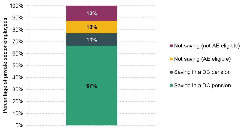
Note: AE = automatic enrolment.
Source: Authors’ calculations using the Annual Survey of Hours and Earnings, 2021.
The other significant group that is not typically in the sample we analyse is employees who are not currently saving in a pension. This is principally because of difficulties with modelling their future saving behaviour. However, given they are not currently saving in a pension, there may well be worries about the levels of their retirement income. Almost a quarter of private sector employees are currently not saving in a pension, split almost equally between those not eligible for automatic enrolment and those who have chosen to opt out of pension saving. Our policy suggestions in Cribb et al. (2024a) include some measures that would boost the retirement saving of this group.
Throughout this report, and the accompanying report on the resulting policy options and our suggestions, in addition to empirical analysis we draw on quotes from individuals interviewed by Ignition House as part of our public engagement work on private pension accumulation conducted as part of the Pensions Review.
The remainder of this report proceeds as follows. Chapter 2 provides a short introduction to the concept of retirement income adequacy and the potential measures of it. Chapter 3 provides an update on some of the influential modelling undertaken by the Pensions Commission on the level of private saving needed for adequate pension incomes. Chapter 4 conducts new modelling using data on individuals’ assets and current saving behaviour to project retirement incomes for current private sector employees, including testing for sensitivity to incorporating partners, housing and inheritances. Chapter 5 provides some additional results from an economic life-cycle model, updating work published in Crawford, O’Brien and Sturrock (2021). A short conclusion is provided in Chapter 6.
2. How to measure adequacy
This report estimates the adequacy of the income that today’s employees will have when they retire. Before we present projections for future retirement incomes, we first consider how we should define and measure income adequacy.
There are different ways of conceiving of retirement income adequacy. These lead to different benchmarks against which to compare retirement incomes and therefore lead to different conclusions about current and future levels of adequacy. This makes it crucial to consider carefully the assumptions behind each concept and benchmark.
There are two broad approaches to conceptualising adequacy. One compares an income with some absolute standard such as a poverty line or particular ‘living standard’. A second approach considers how an individual’s retirement income relates to the income they had during their working life. Both approaches are useful in different ways and so we use them both in our modelling.3
2.1 Poverty line or ‘living standard’ approach
This approach identifies individuals as having adequate resources if their income exceeds a level deemed necessary to purchase a certain standard of living. Previously, work has focused on whether people reach a poverty line (e.g. Crawford and O’Dea, 2012). More recently, with pensioner poverty at much lower levels, and a more comprehensive foundation level of income provided by the new state pension, pensioner poverty in the future – at least for most singles, and couples where both members are above state pension age – is likely to be very low. Cribb et al. (2023a) show that essentially all groups receiving the new state pension in full, but no other income, will be above the poverty line, with the exception of some single people living in the private rented sector in some parts of England.
Perhaps as a result of this, interest has grown in more ambitious metrics that compare individuals’ retirement incomes against a higher fixed income line, most notably the ‘retirement living standards’ benchmarks produced by Padley (2024), based on the Minimum Income Standard benchmark (Padley and Stone, 2023), for the Pensions and Lifetime Savings Association (2024). There are three PLSA retirement living standards levels – minimum, moderate and comfortable – and for each level separate figures are produced for single households and for couple households. The idea of these figures is to give an annual amount of expenditure that achieves a living standard reflective of those terms. Crucially, these expenditure amounts assume no spending on housing costs, care costs or tax. That means that the pre-tax income required to reach those levels will be higher. A household with housing costs – whether mortgage repayments or rental payments – will require a higher income still to reach each benchmark, as will a household that wants to put aside resources to pay for care. Figures for couples are lower (on a per-person basis) because some items can be shared within a household, making it cheaper to achieve a certain standard of living. Separate figures are also produced for those living in London, where costs are expected to be higher.
Other living standard benchmarks exist, on top of poverty lines and the PLSA lines. In particular, the Living Pensions project (Finch and Pacitti, 2021; Cominetti and Odamtten, 2022; Broome, 2024) aims to calculate the size of the pension pot – and corresponding saving rates – needed to meet the Minimum Income Standard benchmark (Padley and Stone, 2023), taking into account both housing costs and income tax. To avoid proliferation of different benchmarks, in this project we focus on the PLSA levels (as well as the replacement rate methodology set out in Section 2.2).
The figures for each PLSA benchmark are produced by researchers in consultation with focus groups. The approach is ‘bottom-up’: the discussions with focus groups aimed to establish which sorts of goods people think are required to reach each of these three standards of living. The total expenditure number is then the cost of acquiring these. Updates in the standards over time reflect both changes in the costs of goods and services and changes in the expectations of retirees about what each standard requires. In 2024, the benchmarks were ‘rebased’ – i.e. established again from scratch – for the first time since their introduction in 2019.
Published in early 2024, the current minimum standard for a single individual is £14,400 per year. The moderate and comfortable standards are £31,300 and £43,100, respectively. The equivalent figures for couples are £22,400, £43,100 and £59,000.
As a definition of retirement income adequacy, these objective benchmarks are helpful in telling us how well off we would expect someone to be and which groups are on track to fall short of a certain standard of living. They are also relatively transparent and easy to interpret and may therefore be helpful for individuals looking to target a particular lifestyle in retirement. This is set out in the following quote from an individual in a focus group considering private pension accumulation undertaken as part of the Pensions Review:
‘I find the retirement living standards easier to understand as it is visual with less information and just the most important. It is easier to refer to and is not overwhelming.’
– Male, aged 45–54
However, living standards benchmarks may, alone, not be a good guide to which groups should be saving more. The reason for that is many households will not reach a given living standard in their working life. In that case, even if they look set to fail to reach a certain benchmark during retirement, it might not be in their best interest to respond by saving more, as it will impact their current standard of living.
This consideration is relevant because the current PLSA retirement living standards are set at rates that many working families do not reach. This is particularly the case for the moderate and comfortable levels, but Figure 2.1 shows that once you take into account people’s housing costs (mortgage repayments or rents), 35% of working households do not reach even the ‘minimum’ standard and 80% do not reach the moderate standard. Single people and those with children are particularly unlikely to meet these levels. In addition, accounting for other costs that working people face but retired people do not, such as childcare costs or commuting costs, would further push up the fraction of working-age people who do not meet these metrics.
Figure 2.1. Share of working households with income net of housing costs below the minimum and moderate PLSA retirement living standards
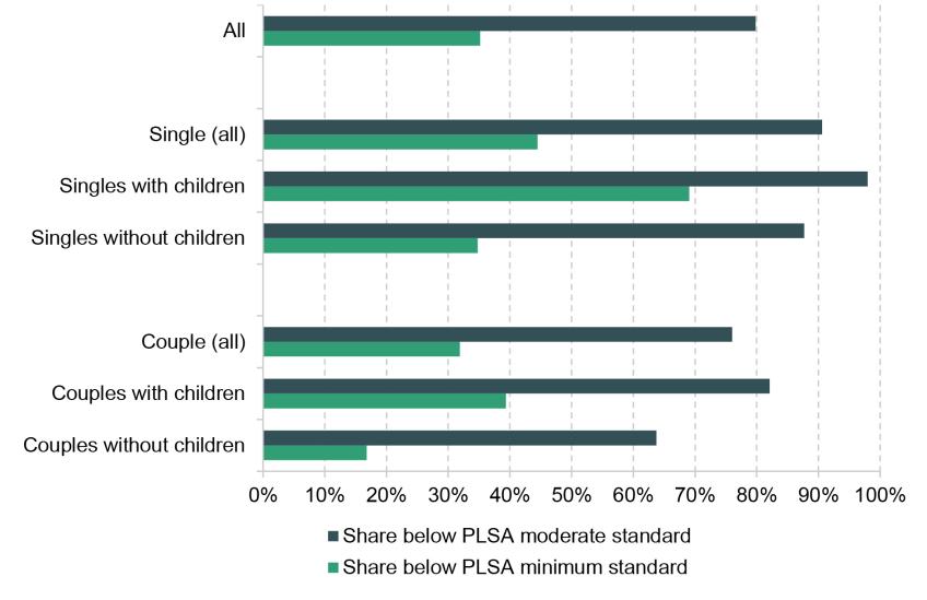
Note: Single/couple households with children have their income equivalised to the level of a single/couple household without children before being compared with the PLSA standards. Equivalisation uses the OECD modified scale. Working-age households with someone in paid work are included.
Source: Authors’ calculations using the Family Resources Survey, 2022–23.
For those households not on track to reach certain living standards benchmarks in retirement but that also have lower living standards in working life than in retirement, increasing private saving may not be the appropriate response. It is still important to measure progress against these benchmarks because this may indicate where other forms of support – most obviously, greater redistribution through either a higher state pension or a more extensive means-tested pensioner benefit system – would be the appropriate response for policymakers with certain distributional preferences. Because the moderate and comfortable living standards are not reached by the vast majority of working-age households, we focus in this report on performance against the minimum benchmark.
One important consideration when measuring projected future retirement incomes against these benchmarks is how they should be assumed to increase over time. Today’s savers presumably should aim to achieve what will be deemed an ‘adequate’ retirement income at the point when they retire, not what was deemed to be adequate sometime in the past. One option would be to increase the PLSA benchmarks in line with inflation. This would embody an assumption that the same basket of goods would be deemed sufficient to meet a minimum/moderate/comfortable living standard in the future. In reality, the basket of goods will also likely change as expectations for minimum living standards rise over time. We assume that these expectations rise in line with living standards in the economy at large, and therefore assume that the PLSA benchmarks rise in line with average earnings over time.
2.2 Replacement rate approach
The replacement rate approach considers retirement income adequate if it maintains a certain proportion of the individual’s pre-retirement income, thus avoiding significant drops in living standards at the point of retirement. This concept is grounded in the idea that people would want to use private saving into pensions to smooth their standard of living over their lifetime. It might be natural to expect that smoothing living standards would mean having the same income in retirement as in working life. However, there are several reasons to expect that a retirement income lower than working-life income can maintain the same standard of living.
First, the same level of expenditure may achieve a higher standard of living in retirement than in working life. Expenses associated with employment, such as commuting and work attire, typically decline or cease entirely at retirement. Housing costs for those buying a home with a mortgage may similarly decline with age. With more free time, retirees might engage more in cost-saving activities such as cooking at home instead of eating out, or shopping around for better prices (Aguiar and Hurst, 2005). That said, some costs – most notably, healthcare and social care costs – tend to rise in retirement, potentially offsetting these other factors.
Second, a given level of expenditure can be achieved with a lower gross income in retirement. One reason for this is that pensioners face a more favourable tax system than those of working age. In particular, pensioners do not pay National Insurance contributions on any of their income, while up to a quarter of any private pension withdrawals can be taken free of income tax. In addition, saving for retirement will end at retirement, meaning that a portion of income is freed up for expenditure.
In principle, we could use empirical evidence to work out what level of income replacement provides a smooth standard of living from working life into retirement. Empirical studies of replacement rates of income in the UK, such as Banks, Blundell and Tanner (1998), find average net replacement rates in the UK around 80%, with higher rates for lower pre-retirement incomes. However, using such studies to set benchmarks requires an assumption that retirees’ incomes are just adequate, which may not always be true. Surveys that seek to elicit desired replacement rates directly, such as Mayhew (2002), reveal varied perceptions. Many on lower incomes desire higher replacement rates, while those on higher incomes often accept lower rates. Binswanger and Schunk (2012) conducted similar studies in the US and the Netherlands, finding that perceived adequate replacement rates decline with higher income levels.
When operationalising replacement rates, one needs to decide over which period to measure retirement and working-life incomes. The perspective of smoothing living standards would suggest looking over the whole of retirement and working life. Often, empirical analysis is restricted by the time frame of datasets and compares the first year of retirement income with some average income over a small number of pre-retirement years. We compare predicted income at retirement with projected pre-retirement incomes, measured at ages 50–59.
Combining theoretical arguments and empirical evidence, there is no single clear definition of an adequate replacement rate. The Pensions Commission (2004) provided one set of benchmark replacement rates. The rates are expressed in terms of gross retirement income as a percentage of pre-retirement gross income and decrease with higher pre-retirement incomes. These are reasonably well established and accepted as useful metrics within the realms of policy and private pensions analysis. We therefore uprate the Pensions Commission benchmarks to today according to earnings growth since 2004, as shown in Table 2.1.
Table 2.1. Target replacement rates for different levels of pre-retirement average earnings
| Target replacement rate | Pre-retirement gross earnings range in 2004 | Pre-retirement gross earnings range in 2023 |
| 80% | £0 to £9,499 | £0 to £16,999 |
| 70% | £9,500 to £17,499 | £17,000 to £31,499 |
| 67% | £17,500 to £24,999 | £31,500 to £44,999 |
| 60% | £25,000 to £49,999 | £45,000 to £89,999 |
| 50% | £50,000 and above | £90,000 and above |
Note: We uprate the pre-retirement gross earnings range from Pensions Commission (2004) based on the change in average weekly earnings for total pay between April 2004 and April 2023 (and then round the resulting earnings ranges). The earnings ranges are then uprated in line with average earnings growth (assumed to be 1.8% per year) for people retiring in future years.
Source: Figure 4.11 in Pensions Commission (2004) and ONS average weekly earnings series EARN01.
These replacement rate benchmarks have limitations and should be used cautiously. They are inevitably somewhat arbitrary. This is particularly the case for higher earners, where changes in the tax system and levels of saving should in principle imply changes in the replacement rates required to smooth living standards. Inevitably, these benchmarks cannot reflect the wide variety in individual circumstances that would be expected to lead to differences in the replacement rate required to smooth living standards. These benchmarks also do not give any indication of when in life any private saving should take place. For these reasons, it can also be useful to look at the outputs from a model that explicitly attempts to calculate what level and timing of saving will smooth living standards and therefore maximise welfare over an individual’s whole lifetime.
The replacement rate benchmarks can be seen as helpful in guiding saving decisions based on the idea of smoothing living standards. As expressed in the quote below, they can be more difficult for some people to understand, given that they are expressed as a percentage of working-life income and do not have an immediate interpretation in terms of a standard of living. Someone reaching adequacy on the replacement rate benchmark can have income that is deemed inadequate by one or more of the living standards benchmarks. These are all reasons for viewing the two types of measure together.
‘From the moment I looked at Replacement Rates my eyes glazed over. Sorry, my issue here! But I am sure lots of other people would feel the same. I like to have financial information presented to me in the simplest of forms, which is done on the Living Standards. I know it’s broad and approximate but I find this so much easier to digest than trying to interpret percentages.’
– Male, aged 45–54
3. What has changed since the Pensions Commission?
When the Pensions Commission reported in the mid 2000s, the landscape for retirement savers was very different from today’s. We therefore update some analysis first conducted for the Pensions Commission to illustrate the implications of the changed saving environment for how much today’s employees might need to save for retirement compared with 20 years ago. We also discuss changes in employer contributions to pensions over time.
3.1 Changes in the landscape for savers
In 2004, a full basic state pension was £79.60 per week, at that point worth 19% of median full-time earnings, equivalent to £139 per week in today’s prices, and it was formally indexed to growth in prices as measured by the Retail Prices Index (RPI). There have been major changes to the outlook for the state pension for today’s savers since 2004, including the introduction of the new state pension for those reaching state pension age from 2016 and the set of reforms implemented from April 2010 that reduced the number of qualifying years needed for a full state pension and treated years spent with certain formal caring responsibilities more favourably. Importantly, the indexation of the state pension is much more generous too, with flat-rate state pensions being indexed in line with the ‘triple lock’ formula since 2011.
The new state pension is paid at a rate depending on the number of years of eligible activities and is much more generous to those with lower levels of earnings than the system it replaced. A full new state pension is now worth £221.20 a week, 59% more in real terms than the basic state pension in 2004 and, at 30% of average full-time earnings, 11% of average earnings more than it was 20 years ago. The DWP forecasts that by the mid 2030s, over 80% of those reaching state pension age will receive a full new state pension (Department for Work and Pensions, 2013). These state pensions will, though, begin to be paid from a later age than may have been expected in 2004, given actual and legislated future increases in the state pension age since then.
Happily, longevity at older ages has improved significantly since 2004. At the time of the Pensions Commission in 2004, a woman aged 65 was expected to live for a further 20.2 years on average. That compares with 21.2 years now expected for a woman aged 65 in 2024. For men, the rise is from 17.4 to 18.6 years. While improvements in longevity have slowed and even showed signs of going into reverse for some groups in recent years (Office for National Statistics, 2024), and there is always significant uncertainty about the future evolution of life expectancy, a central expectation is that people of working age today will tend to live to older ages than was expected 20 years ago for the generation of working-age people then. Longer lives have come alongside more years spent in paid work. At least up until the eve of the pandemic, employment rates for both men and women in their 50s and 60s were rising steadily (Cribb, 2023), with the big rise in the female state pension age one significant factor behind this. Expectations for the number of years spent in retirement for someone retiring at the state pension age have risen from 17.4 to 17.6 for men (despite the one-year increases in the male state pension age from 65 to 66). Given the six-year increase in the state pension age for women, the expected number of years after state pension age for women has fallen from 25.4 to 20.1.
The years leading up to 2004 saw much higher rates of growth in earnings than have been seen since and are now expected in the future. Over the 20 years up until 2004, average annual earnings for someone of working age grew at an annualised rate of 2.8%. Since then, average earnings have barely grown. While some of the poor performance of earnings over the period since 2004 is attributable to economic shocks – most notably, the financial crisis and its aftermath – economists, including the Office for Budget Responsibility (OBR), have consistently downgraded forecasts for future productivity growth, and most long-term expectations are that productivity growth going forward will be lower than over the latter decades of the 20th century.
The final, and perhaps most important, change since 2004 – albeit one closely related to the poor productivity performance mentioned above – is the change in the outlook for returns to saving. Over the 20 years up to 2004, total real returns to UK equities averaged just under 8% per year.4 In the period from 2004 to 2020, they have averaged 4%. The real returns to 15-year government bonds have fallen from a little under 6% per year over the 20 years up to 2004 to 1.5% over the period up to 2020. While UK pension savers do not only save into UK equities and bonds, this illustrates the scale of the changes seen recently. The outlook for returns going forward is of course uncertain. Returns to government bonds have risen substantially in nominal terms in the period since 2022, but the medium-term outlook for the real rate of return to safe assets has changed less. Expectations of financial markets are that real gilt rates will be between 0% and 2% over the coming decades.5
3.2 The implications for required saving rates
We illustrate the importance of this changed saving landscape by estimating the saving rate required to hit a target replacement rate for an individual with certain illustrative earnings levels. These illustrative earnings levels are based on the Pensions Commission analysis and updated to today’s terms.
The calculations are made as follows. We assume that earnings grow at the same rate in each year, and that people work in all years from age 22 until state pension age. We define the individual’s pre-retirement income as their earnings in the year before they reach state pension age, and then multiply this by their target replacement rate (see Table 2.1) to get their target retirement income. We model income at state pension age from state benefits, either following the methodology in Pensions Commission (2004) or, for our updated 2024 analysis, assuming that everyone gets the full new state pension (and no other state benefits). The difference between the individual’s target retirement income and their retirement income from state benefits gives us their target ‘private’ retirement income, and we assume they achieve this by buying an inflation-linked annuity, following the methodology in Pensions Commission (2004). We then calculate the saving rate the individual would need in order to have enough wealth to purchase such an annuity upon reaching state pension age, assuming that the individual saves the same amount in each year of working life.
Key assumptions that feed into this modelling are summarised in Table 3.1. Our earnings growth assumption is line with the OBR’s long-run expected economy-wide earnings growth.6 The assumption on rates of return during accumulation mainly comes from Financial Conduct Authority (2017), although we update the expected rate of return on bonds underlying this calculation in line with current UK gilt curves. To obtain the expected rate of return for annuity providers, we subtract 0.7 percentage points from the return on government bonds (to account for fees). We compare our assumptions with the equivalent ones made by the Pensions Commission in its 2004 analysis.
Table 3.1. Comparison of earnings growth, rate of return, and state pension indexation assumptions
| Pensions Review, 2024 | Pensions Commission, 2004 | |
| Real earnings growth | 1.8% | 2.5% |
| Real rate of return during accumulation | 3.3% | 4.8% |
| Real rate of return for annuity providers | 1.8% | 2.3% |
| Indexation of the state pension | Earnings growth | Inflation |
Note: See Section A.13 for details on our 2024 assumptions. The Pensions Commission assumed an average earnings growth rate of 1.5% above RPI and rates of return of 3.8% above RPI during accumulation and 1.3% above RPI for annuity providers. We assume a wedge of 1 percentage point between the Retail Prices Index and Consumer Prices Index and an average (CPI) inflation rate of 2% per year7 to obtain real rates for the Pensions Commission numbers.
Source: Pensions Commission, 2004.
The results of the analysis are shown in Table 3.2. We show projections for the required saving rates using the Pensions Commission’s assumptions for someone starting their working career at age 22.8 We then show the impact of updating the state pension environment, life expectancy, and rates of return and earnings growth to today’s assumptions. As we work across the columns, the changes are cumulative so that the final column shows the saving rates based on our 2024 assumptions. We show projections for low, middle and high earners (as defined below), all of which are the same levels as shown in Pensions Commission analysis, although uprated in line with average earnings growth to today.
Table 3.2. Required contribution rates to an occupational pension to reach target replacement rates, by earnings, 2004 and 2023
| Earnings (2023 terms) | 2004 environment | Updating state pension | + updating life expectancy | + updating earnings growth and returns: 2023 environment |
| £16,000 | 0% | 2.0% | 2.5% | 3.3% |
| £38,500 | 9.2% | 6.5% | 7.9% | 10.3% |
| £90,000 | 8.5% | 6.4% | 7.7% | 10.0% |
Note: Authors’ calculations updating Pensions Commission (2004) analysis for an individual aged 22 today and working until state pension age. The leftmost column shows their earnings at age 22, which are assumed to grow at a constant rate each year. The individual is assumed to save a constant fraction of their earnings in each year in order to reach their target replacement rate (80% for the lower earner, 67% for the middle earner and 50% for the higher earner). The table shows the saving rate they need to achieve these replacement rates under different economic environments.
Under the 2004 assumptions, the low earner (£16,000 in today’s terms) actually did not need to do any private saving for retirement to meet the target replacement rate benchmark: income from the basic state pension, SERPS (State Earnings-Related Pension Scheme) and pension credit (guarantee credit) were sufficient for them to replace 80% of their pre-retirement earnings.9 Moving to the new state pension system, all else equal, means an increase in the required saving rate for the low earner, due to the loss in SERPS income. In contrast, the middle (£38,500 in today’s terms) and high (£90,000) earners have a required saving rate of around 9% under 2004 assumptions. As a proportion of their pre-retirement income, they receive significantly less income from SERPS and means-tested benefits in retirement than the lower earner. Moving to the new state pension system decreases the required saving rate to around 6.5% as they now receive the new state pension, which we assume is indexed to average earnings growth, meaning a much more generous state pension in the long run than an RPI-indexed state pension as assumed by the Pensions Commission.
Increases in life expectancy push up required saving rates by slightly over 1% of earnings for the middle and higher earners as, essentially, all else equal, longer retirements mean more private saving is needed. Longer life expectancy leads to a much smaller increase in the required saving rate of the lower earner, for whom private saving is a much lower proportion of their retirement income. The lower rates of return and lower growth in earnings lead to an even larger increase in required saving rates, of almost 2.5% of earnings, for the middle and higher earners. The increase is again more muted for the lower earner, who relies much less on private income in retirement. Overall, the increase in required saving rates is larger for the lower earner than for the middle and higher earners, although even today they only have to save a very modest proportion of their earnings.
There is of course significant uncertainty around the future evolution of earnings growth, rates of return and the level of the state pension. Table 3.3 illustrates how our results change when we alter the key assumptions. The rate of return matters for the required saving rates. A 1 percentage point (ppt) higher return and 1ppt higher rate of earnings growth reduces the required saving rate by around 1% of earnings for middle and higher earners. This effect is primarily driven by the change in returns. Changes to the outlook for the state pension matter more for lower earners, as the state pension is a larger proportion of their retirement income. If we assume that the triple lock remains in place (meaning here that the state pension grows 0.58ppts faster than earnings in each year, as assumed by the Office for Budget Responsibility (2023)), this reduces the required saving rate for low and middle earners by around 3% and 2% of earnings, respectively.
Table 3.3. Effect of different assumptions on state pensions and rates of return on required contribution rates to an occupational pension to reach target replacement rates, by earnings
| Earnings | Baseline projection | Higher growth and returns | Lower growth and returns | 10% higher state pension | Triple lock state pension |
| £16,000 | 3.3% | 2.8% | 3.9% | 1.5% | 0% |
| £38,500 | 10.3% | 9.2% | 11.7% | 9.6% | 8.1% |
| £90,000 | 10.0% | 9.0% | 11.3% | 9.7% | 9.1% |
Note: Triple-lock ratchet assumed to be 0.58ppts above earnings indexation as assumed by OBR (2023). Higher/lower earnings growth and asset returns are 1ppt higher/lower compared with the baseline set out in Table 3.1.
Source: Authors’ calculations.
3.3 Changes over time in employer contributions to pensions
Another key trend in the UK pension saving landscape over the last few decades has been the declining prevalence of defined benefit pensions in the private sector. Among private sector employees not working in non-profit institutions, 7% were saving into a defined benefit pension in 2021 (Office for National Statistics, 2022), compared with around 30% in the early 1990s and 35% in the early 1980s (Pensions Commission, 2004). This is important given that employer contributions to defined benefit pensions tend to be substantially higher than contributions to defined contribution pensions.10
Reliable data on employer contributions to pensions in the Annual Survey of Hours and Earnings only go back to 2005, when 24% of all private sector employees were saving in a defined benefit pension. Figure 3.1 shows the aggregate employer pension contribution rate between 2005 and 2021 for private sector employees, calculated as total employer contributions to pensions (excluding one-off payments such as deficit reduction contributions which we discuss below) divided by total gross earnings. Overall, total employer contributions to pensions fell from 5.9% of total earnings in 2005 to 5.1% in the mid 2010s, before rising to 6.0% in 2021 (the latest year for which we have data). This is mainly driven by the fact that many more employees are saving in a workplace pension and receiving an employer contribution now than 20 years ago (though increases in minimum contributions in 2018 and 2019 are likely to have driven some of the rise in the late 2010s).
Figure 3.1. Employer pension contributions to private sector employees’ private pensions, as a percentage of total earnings, split by employer size

Note: Average employer contribution is calculated across all private sector employees, not restricting to those who participate in a workplace pension scheme.
Source: Authors’ calculations using the Annual Survey of Hours and Earnings, 2005 to 2021.
We do not have consistent data before 2005. But the first report of the Pensions Commission (2004) reported a slightly different metric (occupational pension contributions as a percentage of GDP) from the early 1970s to the early 2000s. This has the disadvantage of including public sector and excluding non-occupational DC plans (such as ‘Group Personal Pensions’).11 The Pensions Commission analysis suggests that employer pension contributions rose by about 1% of GDP from the early 1970s to the early 1980s, reaching 2.5% of GDP, before falling to 1% of GDP by the early 1990s, and with a nascent recovery in the late 1990s. It is hard to say exactly where private sector employer pension contributions are (compared with total employee earnings or GDP) relative to recent history given these data limitations – they are certainly at their highest level since the mid 2000s, are probably higher than in the early-to-mid 1990s, but may or may not be as high as they were in the early-to-mid 1980s.
It is also worth looking at how these changes have occurred since 2005, split by employer size. Larger employers were more likely to offer defined benefit pensions in the past, and typically had more of their employees participating in a pension than smaller employers, so we might have expected a drop in their aggregate employer pension contributions as they switched to defined contribution pensions. Despite this, we see that even for the set of employers with at least 1,000 employees, aggregate employer pension contributions were, at 8% of average earnings, around the same level as a fraction of pay in 2021 as they were in 2005. For small employers (fewer than 100 employees), the changes are more marked, particularly in recent years. In 2021, average employer contributions were 3.5% of pay, up from 2.9% in 2005.
These figures only refer to the employer pension contributions made for current employees – they explicitly exclude other employer ‘lump-sum’ contributions to pension schemes. For many years, many employers have had to make ‘deficit reduction contributions’ to their defined benefit pension schemes because of deficits in these schemes. With most private defined benefit schemes closed to new accrual (or at least to new members), these payments helped secure the retirement incomes of (mostly) current pensioners or other previous employees, rather than being a form of remuneration for current work of employees.
However, there have been large falls in these payments in recent years. Data from the Pension Protection Fund (2024) show that the fraction of defined benefit schemes in deficit has fallen from around 60% in 2020 to below 10% in 2024 as nominal interest rates have risen, which has cut pension scheme liabilities by more than the fall in the value of their assets. Data from HM Revenue and Customs (2024) show that the tax relief applied to deficit reduction payments fell from £5.1 billion in 2020–21 to £2.8 billion in 2022–23 as interest rates rose.
There is some evidence on how the obligation to fill pension deficits affects firms and workers. Adrjan and Bell (2018) find that most of the burden has fallen on the firms themselves, although there was evidence of some incidence on employees’ wages (about 10% of the cost of deficit payments fed through into lower wages). If there is symmetry in the responses to the (broadly unexpected) decline in pension deficits over the last few years, then we would in general expect firms (and therefore shareholders) to be the key beneficiary from the reduction in pension deficits, but employees to benefit modestly too through slightly higher wages.
3.4 Summary
There have been substantial changes to the pension saving environment since 2004, including reforms to the state pension system, increases in life expectancy, and lower expected rates of return and earnings growth rates. The analysis in this chapter suggests that, in all, these changes likely mean that people would need to do slightly more saving for retirement than suggested in the Pensions Commission reports, by slightly over 1% of earnings for middle and higher earners. This is driven by increases in life expectancy and lower expected rates of return on saving. We also find that lower earners might need to do more private saving for retirement today than in the world as it was 20 years ago to hit target replacement rates; however, in both periods, required saving rates are very low as the state replaces a large proportion of pre-retirement earnings.
Importantly, there is a significant degree of uncertainty about future earnings growth, rates of return and the level of the state pension, and our assumptions on how much people need to save are relatively sensitive to assumptions about these parameters. Employers are contributing more (as a fraction of total earnings) to their employees’ private pensions in 2021 than in 2005. This is particularly the case for smaller employers (who in the past will have been less likely to offer relatively generous defined benefit pensions and more recently will have been more greatly affected by automatic enrolment), but is also the case amongst larger employers.
4. What is the outlook for adequacy on current trends?
As discussed in the previous chapter, changes in the saving landscape – in particular, a lower expected rate of return on pension saving and higher life expectancy – mean that people will generally have to save more to hit their target replacement rates than was the case 20 years ago. Of course, there have also been large changes in how much employees are saving for their pension since the early 2000s, due to, for example, automatic enrolment.
In this chapter, we therefore take stock of the pension saving position of current private sector employees. As explained in Chapter 1, we mostly focus on our main sample of private sector employees, aged 25–59, currently saving in a defined contribution pension. The focus on those saving in DC pensions means our work is comparable to that of others who have undertaken similar exercises, such as Pike (2022).
In this chapter, we document the distributions of pension saving and pension wealth among this group, and how these vary with earnings and age. Then we undertake new modelling to project future retirement incomes for our sample of interest, highlighting the uncertainty associated with our estimates, and how the results differ for different groups and with different modelling assumptions. Throughout, we compare these projected future retirement incomes with both the incomes needed to hit target replacement rates and the PLSA minimum retirement living standard, as described in Chapter 2.
4.1 Current trends in pension saving
Before diving into the modelling, we first show the distributions of both current pension wealth and pension contribution rates among our analysis sample in Round 7 of the Wealth and Assets Survey. We uprate wealth to 2023 prices using the Consumer Prices Index.
Figure 4.1 shows the distribution of total private pension wealth (including both defined contribution and defined benefit pension wealth) by age.12 Clearly, there is a wide dispersion in the amount of private pension wealth that employees have accumulated to date. Around 40% of private sector employees currently saving in a DC pension have accumulated less than £10,000 of pension wealth, while another 20% have pension wealth of over £100,000. Unsurprisingly, younger employees are particularly likely to have low levels of pension wealth, with almost two-thirds of 25- to 34-year-olds having pension wealth of less than £10,000. However, even among 50- to 59-year-old employees, over one in five have less than £10,000 in pension wealth. On the other hand, more than a quarter of this older age group have pension wealth of over £250,000. This highlights that the dispersion of pension wealth is particularly wide among those in their 50s; some of these employees will have missed out on many years of pension saving as pension participation fell during the 2000s, while others might have accrued a large defined benefit pension either from a private sector employer (when these schemes were more prevalent) or from a spell working in the public sector.
Figure 4.1. Distribution of total pension wealth among private sector employees saving into a DC pension, by age group

Note: Sample contains private sector employees aged between 25 and 59 currently saving into a defined contribution pension. Pension wealth is uprated to April 2023 prices.
Source: Authors’ calculations using Round 7 of the Wealth and Assets Survey.
Figure 4.2 shows the distribution of pension wealth for different quartiles of the current earnings distribution. There is again a large spread of pension wealth among middle and, especially, higher earners. A quarter of those earning more than £59,000 annually have pension wealth of less than £25,000, while another quarter have pension wealth of over £250,000. Lower earners typically have lower levels of pension wealth than higher earners, as expected.
Figure 4.2. Distribution of total pension wealth among private-sector employees saving into a DC pension, by current earnings quartile
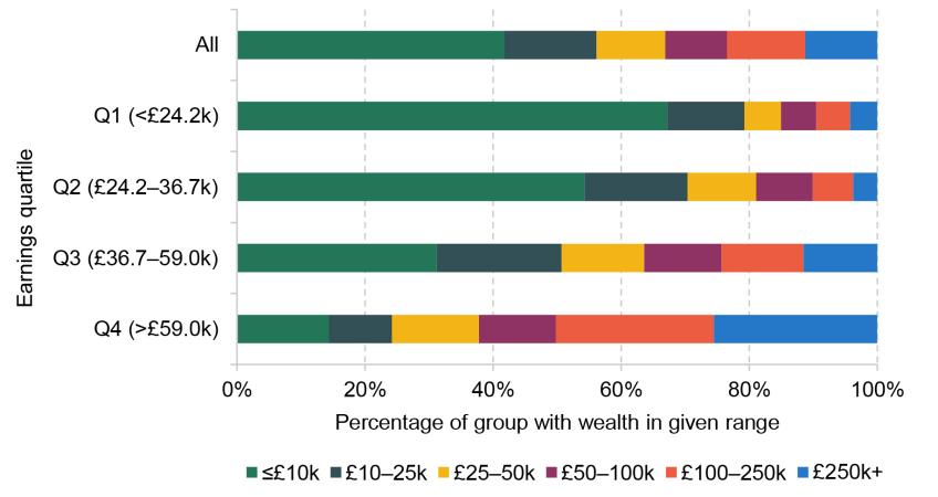
Note: Sample contains private sector employees aged between 25 and 59 currently saving into a defined contribution pension. Pension wealth is uprated to April 2023 prices.
Source: Authors’ calculations using Round 7 of the Wealth and Assets Survey.
Of course, earnings and age are related: employees in their 50s tend to earn more than those at the start of their career. Table 4.1 therefore shows median total pension wealth in our sample by both age group and earnings quartile. This highlights that the patterns in Figures 4.1 and 4.2 are not driven solely by earnings or solely by age, but that both are important for pension wealth. For a given level of earnings, older workers tend to have higher pension wealth, while for a given age group, higher earners tend to have higher pension wealth. Median pension wealth is just £1,800 among lower earners aged between 25 and 34, compared with around £280,000 for higher earners in their 50s.
Table 4.1. Median total pension wealth among private sector employees saving into a DC pension, by age group and earnings quartile
| Earnings quartile | Age 25–34 | Age 35–49 | Age 50–59 | All |
| Q1 (<£24.2k) | £1,800 | £4,200 | £19,600 | £3,700 |
| Q2 (£24.2–36.7k) | £3,900 | £11,500 | £38,200 | £7,800 |
| Q3 (£36.7–59.0k) | £8,900 | £34,800 | £114,900 | £24,200 |
| Q4 (>£59.0k) | £23,500 | £120,500 | £278,000 | £101,000 |
| All | £4,800 | £26,300 | £77,000 | £17,000 |
Note: Sample contains private sector employees aged between 25 and 59 currently saving into a defined contribution pension. Pension wealth is uprated to April 2023 prices. Figures rounded to the nearest £100.
Source: Authors’ calculations using Round 7 of the Wealth and Assets Survey.
Figures 4.3 and 4.4 show the corresponding relationships between current total (employee + employer) pension contribution rates, as a proportion of gross pay, and age and earnings. Again, there is substantial variation in pension contribution rates; however, there is much less correlation between contribution rates and earnings or age than for pension wealth.
Figure 4.3. Distribution of total pension contribution rates (% of earnings) among private sector employees saving into a DC pension, by age group
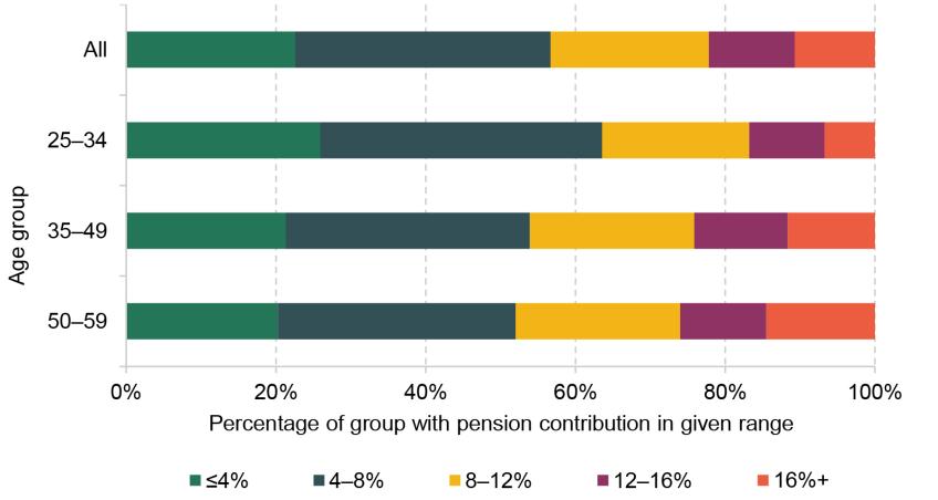
Note: Sample contains private sector employees aged between 25 and 59 currently saving into a defined contribution pension. Total pension contribution rates are calculated as employee + employer pension contributions divided by total (gross) earnings.
Source: Authors’ calculations using Round 7 of the Wealth and Assets Survey.
Figure 4.4. Distribution of total pension contributions (% of earnings) among private sector employees saving into a DC pension, by current earnings quartile
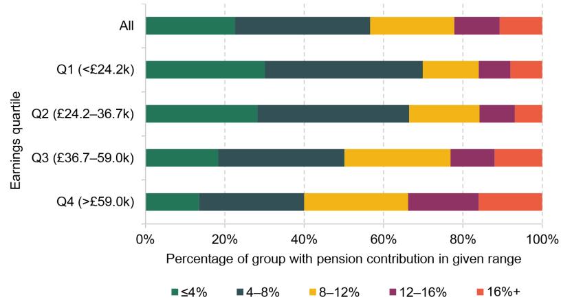
Note: Sample contains private sector employees aged between 25 and 59 currently saving into a defined contribution pension. Total pension contribution rates are calculated as employee + employer pension contributions divided by total (gross) earnings.
Source: Authors’ calculations using Round 7 of the Wealth and Assets Survey.
One thing that stands out from these figures is that a significant fraction of private sector employees saving in DC pensions have low contribution rates. Over 20% are contributing at most 4% of total earnings, and over half are contributing no more than 8% of total earnings. On the other hand, nearly a quarter have a contribution rate of over 12% of earnings. Older employees are slightly more likely to have higher contribution rates than those aged between 25 and 34, and higher earners also tend to have higher contribution rates than lower earners. Indeed, almost 70% of those in the bottom half of the earnings distribution are contributing at most 8% of earnings to their pension.
Despite this, we still find that the share contributing less than or equal to 8% of earnings to their pension is 45% among those in the top half of the distribution, and 52% among those aged between 50 and 59. Even among those in the top half of the distribution and aged between 50 and 59, 36% have a contribution of at most 8% of earnings. This is likely a particularly good time in working life for many of these individuals to do their pension saving, when their earnings are high and when their outgoings are often lower due to lower mortgage repayments and lower childcare costs (Crawford, O’Brien and Sturrock, 2021).
It is important to remember that the previous graphs in this section on pension contributions have focused on the sample of private sector employees saving in a defined contribution pension. As emphasised in Chapter 1, there are also many private sector employees who are not currently contributing to a pension at all. Figure 4.5 shows that, overall, 27% of all private sector employees are not saving in a pension in Round 7 of the Wealth and Assets Survey, with around half of these non-savers eligible for automatic enrolment (and therefore, presumably, opting out of their workplace pension) and half not eligible.
Figure 4.5. Percentage of working-age private sector employees not saving in a pension, by automatic enrolment eligibility and group

Note: AE = automatic enrolment. SPA = state pension age. The sample contains all private sector employees aged between 16 and 63 (for women) and between 16 and 64 (for men), inclusive, in Round 7 of the Wealth and Assets Survey.
This graph also shows the share not saving in a pension for different groups of private sector employees. Those aged between 16 and 24 are particularly likely to be ineligible for automatic enrolment and not saving in a pension, which is unsurprising given that the current lower age limit for automatic enrolment eligibility is 22. Private sector employees aged between 60 and state pension age are also slightly more likely not to be saving in a pension than those of other ages, both due to slightly higher rates of ineligibility (with many working part-time earning below the earnings trigger) and of opting out. Over half (54%) of those in the bottom quarter of the earnings distribution are not saving in a pension, with most of them not eligible for automatic enrolment (principally due to the £10,000 earnings trigger). In addition, women are more likely not to be saving in a pension than men as they are less likely to be eligible for automatic enrolment, consistent with results in Cribb, Karjalainen and O’Brien (2023). Groups with lower levels of formal education qualifications are more likely not to be saving in a pension, as are part-time workers compared with full-time workers. All these results on who is not saving in a pension are important to keep in mind when interpreting the modelling results, which focus on the sample of 25- to 59-year-old private sector employees currently contributing to a defined contribution pension. We do show results for the sample of all private sector employees (who are not saving in a defined benefit pension) in Table B.3 in Appendix B, but we do not include non-pension-savers in our main sample given more uncertainty about how their pension saving might evolve in the future.
4.2 Overview of modelling approach
Our modelling takes the current position of employees and projects forward the retirement incomes they may expect on current trends. In this section, we provide a high-level overview of how this modelling works and the main assumptions we have made. Appendix A contains a full, self-contained, description of the modelling.
The underlying data for our model come from the Wealth and Assets Survey (Round 7), where respondents report their earnings, total pension wealth, current pension contribution rate, sex, age and education level. We simulate forward earnings and employment for each employee until they permanently leave the labour force. These simulations are based on observed data from Understanding Society (also known as the UK Household Longitudinal Survey), and we allow people with different education levels, people from different generations, and men and women to have different earnings trajectories. Our method allows people to move up and down the earnings distribution and to move into and out of paid work in a way broadly consistent with what has happened in the past. In addition, the earnings processes are consistent with future economy-wide earnings growth of 1.8% per year, in line with OBR long-term assumptions.
As well as allowing for movements into and out of paid work during working life, we also model when people permanently leave the labour force. We assume that people aim to retire at state pension age; however, some people are forced to retire earlier than this (as early as age 60) – for example, due to health problems, because they have to care for a family member or because they lose their job and are unable to find another one. We do not allow people to work past state pension age in our modelling, nor do we allow people to retire before state pension age because they think they have already accumulated enough wealth to enjoy a comfortable standard of living in retirement.
We assume that people save a constant fraction of their earnings – as defined by their current total (employer + employee) contribution rate – into their pension in all future years in which they are in paid work. People then access their pension pot (coming from any defined contribution wealth they had already accumulated by the time they were surveyed, plus future saving, plus returns they get on their saving) once they permanently leave the labour force. An individual’s retirement income is calculated in the first year after they permanently leave work. As well as their defined contribution pension income, an individual’s retirement income will also be made up of either state pension income or means-tested state support (depending on whether they leave work at state pension age or earlier), any defined benefit income they had already accrued rights to in a previous job, and, in some specifications, annuitised income from other forms of wealth (e.g. from future receipt of inheritances or existing financial wealth held outside of pensions).
We assume all pensioners receive a full new state pension from state pension age. If someone leaves paid work before state pension age, we assume they draw down their defined contribution (and other) wealth more quickly in the period before they reach state pension age, before annuitising the rest upon reaching state pension age in order to smooth their income over their whole retirement. The state pension is assumed to grow in line with average earnings (1.8% per year in real terms) in the baseline model, while the generosity of working-age means-tested support is increased in line with prices.
We then compare the individual’s projected retirement income with a given measure of adequacy. The PLSA minimum retirement living standard is worth £14,400 per year currently; we convert this to a pre-tax measure and then uprate it in line with average earnings – this implicitly assumes that society’s view of a minimum acceptable standard of living in retirement (as judged by this measure) rises as the country becomes more prosperous. For the target replacement rate measure of adequacy, we define pre-retirement income as the individual’s average income between ages 50 and 59. We then multiply this by the relevant target replacement rate to get a measure of target retirement income (the target replacement rates are outlined in Chapter 2 – see Table 2.1).
As well as assessing whether an individual’s projected retirement income is on track to hit a given measure of adequacy on current trends, we can also calculate the share of future earnings that they would need to save in order to reach adequacy under different metrics. In addition, we can project what might happen to their retirement income if parameters of the automatic enrolment system were changed, such as an increase in minimum default contribution rates.
In an extension to the model, we also show what happens if we model individuals as couples rather than as individuals, assuming that earnings and retirement resources are shared equally between both members. To do this, we focus on people aged at least 35, given that the share of people with a cohabiting partner or spouse is much less stable before this age, and we assume that couples remain married/partnered at least until retirement.13 When doing this, we compare single people with the PLSA minimum retirement living standard for single people and we compare couples with the PLSA standard for couples.
We also show the potential effect of future inheritance receipt on projected retirement incomes and the shares reaching adequacy. To do this, we model people as receiving an inheritance from a distribution consistent with previous work by IFS researchers (Bourquin et al., 2020) depending on their education level, their generation and whether their parents are homeowners – see Figure A.1 in Appendix A for the distribution of inheritances received in our model. We assume inheritances are received at age 60 and are used to fund their retirement living standards. This can be thought of as an upper bound of the effect of inheritances – for example, some may decide to pass the wealth on to their children.14
In another extension, we account for the extra living costs brought about by private renting in retirement. To do this, we assume that anyone aged at least 45 who rents their home privately in the survey will also be a private renter in retirement. For private renters aged between 35 and 44, we estimate the probability of moving out of private renting for this age group based on data from Understanding Society, where we allow the probability to vary by earnings, region and marital status. We then scale these probabilities such that the overall private renting share for this age group matches the overall private renting share for people born in the early 1970s. Once we have determined who will be privately renting in retirement, we adjust our measures of target retirement income for these individuals and calculate the share who reach these adjusted targets, taking into account that some renters will receive housing benefit which will cover at least part of their rent.
As noted in Chapter 2, there have been several other attempts to model future retirement incomes, such as Pike (2022) and Department for Work and Pensions (2023) in recent years. As well as sharing similarities, the modelling in all these reports differ in several important ways. Different modellers make different assumptions about how various factors might evolve in the future, and make fundamentally different choices about how to model the world. Despite this, many of the results in this report are broadly consistent with these previous modelling exercises, lending credibility to our (and, by extension, their) results.
4.3 Projections at the individual level
We first set out the baseline results from our modelling. This is for our entire sample of 25- to 59-year-old private sector employees saving into a DC pension, modelled at the individual (rather than couple) level, and without taking into account housing costs or the possibility of receiving an inheritance. Our baseline assumptions for how the economy will evolve in the future are as in Chapter 3: average real earnings growth is assumed to be 1.8% per year, people achieve a real rate of return of 3.3% per year on pension saving during the accumulation phase, and the real rate of return during the decumulation phase (used for calculating annuity rates) is 1.8%. The state pension is assumed to be indexed in line with average earnings growth.
Figure 4.6 shows that, in this baseline model, 57% of our sample are on track to hit their target replacement rate and 68% are on track to achieve the PLSA minimum retirement living standard. In other words, over two in five individuals (7 million people) are projected to be ‘undersaving’ relative to the target replacement rate metric, and one in three (5 million) are relative to the PLSA minimum metric. So in both cases a substantial minority appear to be undersaving.
Figure 4.6. Percentage of private sector employees saving into a DC pension who are projected to hit different measures of retirement income adequacy, by group

Note: The sample contains 25- to 59-year-old private sector employees saving into a DC pension in Round 7 of the Wealth and Assets Survey. We simulate their projected future retirement income under our baseline assumptions, modelling everyone at the individual level and without accounting for future housing costs or inheritances. We then compare these future retirement incomes with the two measures of retirement income adequacy. Earnings quartiles are based on pre-retirement earnings, i.e. simulated average earnings between ages 50 and 59.
This graph also highlights that the groups projected to achieve ‘adequacy’ are quite different for the two metrics, especially when we look at the patterns by earnings. On the one hand, over 85% of those in the bottom quartile of pre-retirement earnings are on track to achieve their target replacement rate, compared with only around 40% of those in the top quartile. In contrast, only 38% of those in the lowest pre-retirement earnings quartile are on track to hit the PLSA minimum retirement living standard, compared with over 90% in the top quartile.
This difference fundamentally arises because target retirement incomes are higher for those with higher pre-retirement earnings under the target replacement rate metric, while the PLSA minimum retirement living standard does not vary with earnings. Higher earners find it easier to reach the minimum standard because relatively low pension saving rates might still be sufficient for them to reach this benchmark, which will not be the case for lower earners. The proportion achieving their target replacement rate is particularly high for lower earners because they almost replace a sufficient proportion of their pre-retirement income with the state pension alone. In fact, the only lower earners who do not reach their target replacement rate on this measure are those who have to leave work before state pension age. These people do not have any state pension income in their measured retirement income, since we measure these in the first year after permanently leaving the labour force. Once they reach the state pension age, the value of a new state pension is sufficiently large relative to their earnings when working for their replacement rate to be reached.
There are further differences in the patterns of who reaches adequacy between the two metrics, principally driven by differences in earnings between different subgroups. Women, who tend to earn less than men, are slightly more likely to reach their target replacement rate but are less likely to reach the PLSA minimum retirement living standard. Similarly, a higher proportion of part-time workers than full-time workers achieve their target replacement rate, while a lower proportion reach the PLSA minimum standard. Interestingly, the proportions hitting both types of adequacy vary little with age.
Figure 4.6 also shows that people who have to leave work before state pension age are particularly unlikely to reach the PLSA minimum retirement living standard. There are several reasons for this. First, they have fewer years of working life over which to accumulate private pension wealth. Second, we assume in the model that people who have to leave work before state pension age make use of their private pension wealth to boost their consumption in the years between leaving paid work and reaching state pension age, given that the UK has a significantly more generous state benefit system for people over state pension age than for people just under. As a result, many of these people are assumed to use up a lot of their private pension wealth in the years before reaching state pension age. Finally, we measure retirement incomes in the first year after permanently leaving paid work. Some people leaving paid work permanently before state pension age will have particularly low incomes at this point, if they have accumulated little private pension wealth and have to rely only on state benefits at this point. They would then have an increase in income once they hit state pension age, although given that the level of the state pension is below the level of the PLSA minimum standard, they would still fail to reach this measure of adequacy at that point. On the other hand, we see that people in this group are not particularly unlikely to meet their target replacement rates. This is because the group also tends to have very low incomes in their 50s. Policies to help these people stay in work for longer would boost both their retirement incomes and their incomes in their 50s, and would mean they do more years of saving and draw down less of their accumulated private pension wealth before reaching state pension age.
In Table B.3 in Appendix B, we replicate Figure 4.6 for two other samples: the sample of 25- to 59-year-old employees who are currently saving into a defined benefit pension, and the sample of 25- to 59-year-old private sector employees who are not currently saving into a defined benefit pension. Overall, 79% of employees saving into a defined benefit pension are on track to hit their target replacement rate and 86% are on track to hit the PLSA minimum retirement living standard. These shares are significantly higher than in Figure 4.6, reflecting that these pensions are typically more generous than defined contribution pensions, especially due to particularly high employer contributions. All groups have relatively high levels of adequacy, except for the group who have to leave work before state pension age, and we still to some extent see a similar pattern with respect to earnings as in Figure 4.6. Among the set of private sector employees not saving into a defined benefit pension, we see lower levels of adequacy than in Figure 4.6, as the sample now contains those who are not currently saving into a pension. Given that we assume that people will always contribute the same amount of their earnings into a pension as currently, these people accumulate no further pension wealth in the future and are unlikely to hit either measure of adequacy. This may not be a particularly realistic assumption, as we might expect this group to start to save in a pension at some point, which is why we have not included them in our main analysis sample. Nevertheless, the incomes of this group in retirement clearly still remain a concern.
Of course, while whether someone reaches a given measure of adequacy is a binary question, it is important to ascertain how close to or far away from the target metric their incomes are. If everyone not reaching adequacy was only £1 away from reaching their target, we would have far fewer concerns than if everyone needed a much bigger boost in their retirement incomes to reach adequacy.
In Figure 4.7, we plot the empirical cumulative distribution function (CDF) of projected retirement incomes (deflated by earnings to 2023 values) for our main sample of interest, private sector employees currently saving in a defined contribution pension. Each line shows what share of the group have projected retirement income lower than the value on the horizontal axis. The dashed vertical line shows the value of the PLSA minimum retirement living standard (just under £15,000 a year in pre-tax terms). So, for example, we can see that the grey ‘All’ line, crosses this dashed line at 32%, which corresponds to the share of the sample not reaching this PLSA metric in Figure 4.6. We can read up from any other value of retirement income on the horizontal axis to similarly get the proportion of the group with retirement income lower than this value. The different colour lines show the empirical CDFs for different quartiles of pre-retirement earnings.
Figure 4.7. Distribution of projected retirement incomes among private sector employees saving into a DC pension, by quartile of earnings
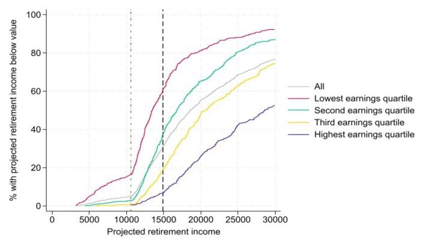
Note: The sample contains 25- to 59-year-old private sector employees saving into a DC pension in Round 7 of the Wealth and Assets Survey. We simulate their projected future retirement income under our baseline assumptions, modelling everyone at the individual level and without accounting for future housing costs or inheritances. The graph then plots the empirical cumulative distribution function of retirement incomes, deflated to 2023 by average earnings growth, separately for four quartiles of average earnings between ages 50 and 59. The dashed vertical line shows the value of the (pre-tax) PLSA minimum retirement living standard. The green dashed-and-dotted vertical line shows the value of the new state pension. We limit the horizontal axis to values from 0 to £30,000.
Two things stand out from Figure 4.7. First, unsurprisingly, those in the top pre-retirement earnings quartile are not only very likely to reach the PLSA minimum retirement living standard, but a sizeable proportion are projected to have much higher retirement incomes than this. In fact, around one in three are forecast to reach the PLSA moderate retirement living standard.
The second thing that stands out from Figure 4.7 is the importance of the state pension for the retirement incomes of, in particular, the lowest pre-retirement earnings quartile. Although only two in five of this group are on track to have retirement incomes above the PLSA minimum retirement living standard, nearly half of the lowest quartile are projected to have incomes between the state pension and this PLSA standard. Again, this highlights the importance of the state pension for the retirement living standards of lifetime low earners. However, over 15% of this group (around 650,000 individuals) have initial incomes in retirement below the value of the state pension. These are individuals who our modelling suggests will have to leave work before state pension age, and who will not have enough pension wealth accumulated by the time of their labour force exit to be able to top up their incomes to at least the value of the state pension before they reach state pension age. These people will experience an increase in their retirement incomes once they reach state pension age and therefore start to receive the new state pension (which is not reflected in our calculations since we focus on retirement incomes in the first year after permanently leaving work), but they have particularly low incomes in the period just before reaching state pension age.
Figure 4.8 shows the empirical cumulative distribution functions of the ratio of projected retirement income to target retirement income under the target replacement rate measure for our main sample. Reading up the dashed vertical line to the grey ‘All’ line shows that 43% have a ratio of projected to target retirement income of less than 1, i.e. 57% are on track to have a retirement income higher than their target replacement rate income (as in Figure 4.6).
Figure 4.8. Distribution of ratio of projected retirement income to replacement-rate-target retirement income among private sector employees saving into a DC pension, by quartile of earnings
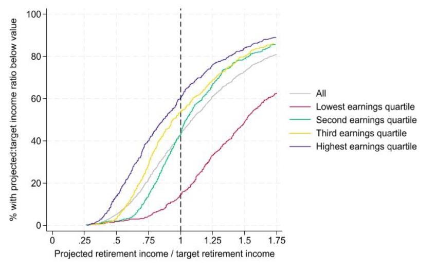
Note: The sample contains 25- to 59-year-old private sector employees saving into a DC pension in Round 7 of the Wealth and Assets Survey. We simulate their projected future retirement income under our baseline assumptions, modelling everyone at the individual level and without accounting for future housing costs or inheritances. The graph then plots the empirical cumulative distribution function of projected retirement income divided by target retirement income (based on their replacement rate), separately for four quartiles of average earnings between ages 50 and 59. We limit the horizontal axis to values from 0.25 to 1.75.
Consistent with Figure 4.6, we get different patterns in Figures 4.7 and 4.8 by earnings quartile. The proportion not reaching their target replacement rate is much lower among those in the lowest quartile of pre-retirement earnings than among those in higher quartiles. This is because those in the lowest quartile have much lower target retirement incomes under this metric, and a full new state pension gets them most, or all, of the way there on its own. In fact, nearly 40% of those in the bottom pre-retirement earnings quartile have a retirement income of at least 175% of their target replacement rate income.
Figures 4.9 and 4.10 show the analogous empirical CDF figures for different age groups, while Figures 4.11 and 4.12 show the analogous figures for men and women separately. Although the shares of each age group reaching the PLSA minimum living standard are similar, Figure 4.9 suggests that projected retirement incomes will be more dispersed among those in their 50s. The distributions of projected retirement incomes divided by target-replacement-rate incomes are more similar for the three age groups.
Figure 4.9. Distribution of projected retirement incomes among private sector employees saving into a DC pension, by age group
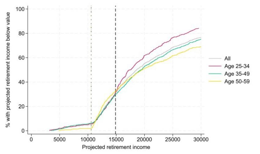
Note: The sample contains 25- to 59-year-old private sector employees saving into a DC pension in Round 7 of the Wealth and Assets Survey. We simulate their projected future retirement income under our baseline assumptions, modelling everyone at the individual level and without accounting for future housing costs or inheritances. The graph then plots the empirical cumulative distribution function of retirement incomes, deflated to 2023 by average earnings growth, separately for three (current) age groups. The dashed vertical line shows the value of the (pre-tax) PLSA minimum retirement living standard. The green dashed-and-dotted vertical line shows the value of the new state pension. We limit the horizontal axis to values from 0 to £30,000.
Figure 4.10. Distribution of ratio of projected retirement income to replacement-rate-target retirement income among private sector employees saving into a DC pension, by age group
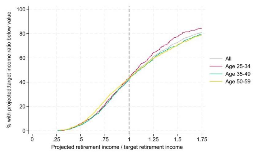
Note: The sample contains 25- to 59-year-old private sector employees saving into a DC pension in Round 7 of the Wealth and Assets Survey. We simulate their projected future retirement income under our baseline assumptions, modelling everyone at the individual level and without accounting for future housing costs or inheritances. The graph then plots the empirical cumulative distribution function of projected retirement income divided by target retirement income (based on their replacement rate), separately for three (current) age groups. We limit the horizontal axis to values from 0.25 to 1.75.
Figure 4.11 shows that women are projected to have lower retirement incomes than men throughout the distribution. This is both because they tend to have lower earnings and because they typically spend more time out of the labour force. Indeed, as women are more likely than men to have to leave work before state pension age, they are twice as likely as men to have modelled income lower than the value of the state pension in the first year after leaving work. In contrast, Figure 4.12 shows that women are slightly more likely than men to achieve their target replacement rate throughout the distribution, driven by the fact that they on average have lower earnings, and those with lower lifetime earnings are more likely to achieve their target replacement rate.
Figure 4.11. Distribution of projected retirement incomes among private sector employees saving into a DC pension, by sex
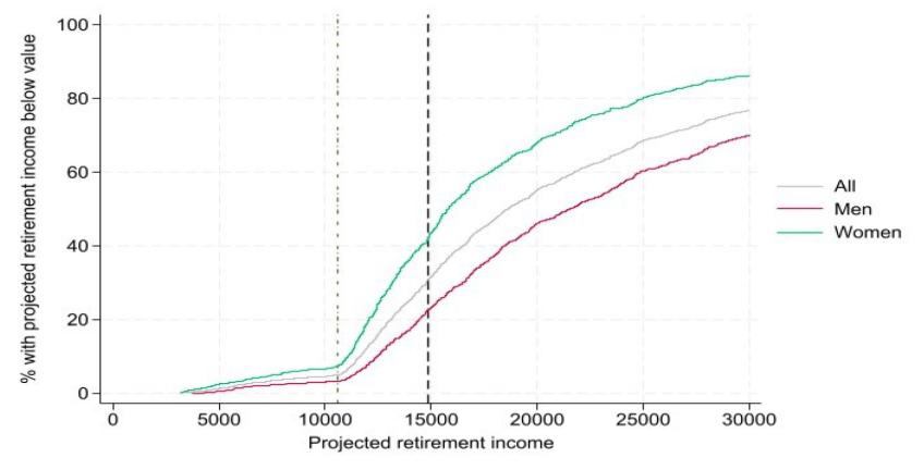
Note: The sample contains 25- to 59-year-old private sector employees saving into a DC pension in Round 7 of the Wealth and Assets Survey. We simulate their projected future retirement income under our baseline assumptions, modelling everyone at the individual level and without accounting for future housing costs or inheritances. The graph then plots the empirical cumulative distribution function of retirement incomes, deflated to 2023 by average earnings growth, separately for men and women. The dashed vertical line shows the value of the (pre-tax) PLSA minimum retirement living standard. The green dashed-and-dotted vertical line shows the value of the new state pension. We limit the horizontal axis to values from 0 to £30,000.
Figure 4.12. Distribution of projected ratio of retirement income to replacement-rate-target retirement income among private sector employees saving into a DC pension, by sex
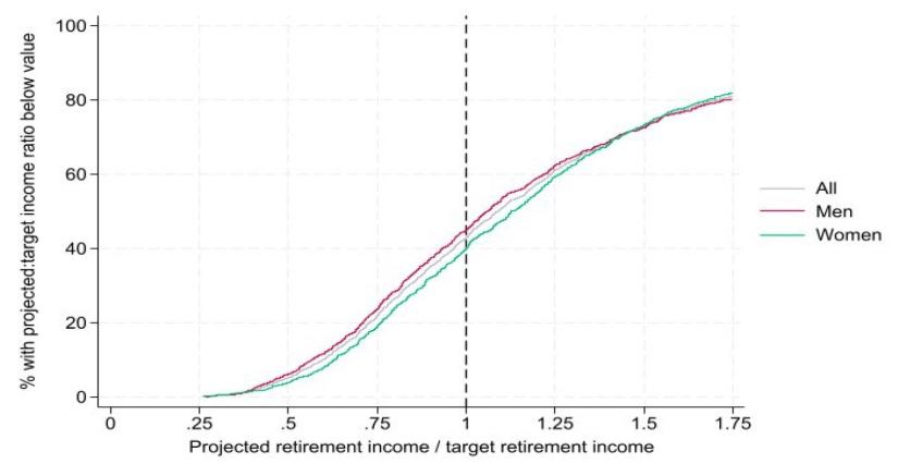
Note: The sample contains 25- to 59-year-old private sector employees saving into a DC pension in Round 7 of the Wealth and Assets Survey. We simulate their projected future retirement income under our baseline assumptions, modelling everyone at the individual level and without accounting for future housing costs or inheritances. The graph then plots the empirical cumulative distribution function of projected retirement income divided by target retirement income (based on their replacement rate), separately for men and women. We limit the horizontal axis to values from 0.25 to 1.75.
In addition to forecasting retirement incomes, we can also use the model to calculate what fraction of future earnings people would have to save in order to reach a given measure of adequacy, under the assumption that they save a constant fraction of earnings in each year. This can help guide us as to whether the default rates under automatic enrolment might be set at the appropriate level to help people save enough to reach a given target.
Table 4.2 displays the median required pension contribution rate, as a percentage of total gross earnings, needed to reach each measure of adequacy, separately for all our sample and for ‘undersavers’ (i.e. those not on track to reach the given adequacy measure). The first row shows that, among our whole sample, the median required saving rate to achieve their target replacement rate is 6%, while the median required rate to achieve the PLSA minimum retirement living standard is 3%. The required rates for undersavers are significantly higher, at 14% and 12% respectively.
Table 4.2. Median required pension contribution rate, as a percentage of earnings, to achieve an adequate retirement income for everyone and those currently not on track to achieve adequacy, by age group and quartile of earnings between ages 50 and 59
| Age group | Age 50–59 earnings quartile | Everyone | Undersavers | ||
| Target replacement rates | PLSA minimum RLS | Target replacement rates | PLSA minimum RLS | ||
| All | All | 6% | 3% | 14% | 12% |
25–34 35–49 50–59 | All All All | 7% 6% 3% | 3% 3% 0% | 11% 14% 27% | 8% 11% 20% |
25–34 35–49 50–59 | Q1 Q1 Q1 | 0% 0% 0% | 9% 11% 18% | 7% 10% 19% | 16% 17% 32% |
25–34 35–49 50–59 | Q2 Q2 Q2 | 5% 6% 10% | 4% 4% 5% | 7% 11% 21% | 6% 9% 14% |
25–34 35–49 50–59 | Q3 Q3 Q3 | 8% 10% 15% | 3% 1% 0% | 10% 14% 27% | 6% 9% 14% |
25–34 35–49 50–59 | Q4 Q4 Q4 | 13% 12% 15% | 2% 0% 0% | 14% 17% 32% | 3% 5% 8% |
Note: RLS = retirement living standard. The sample contains 25- to 59-year-old private sector employees saving into a DC pension in Round 7 of the Wealth and Assets Survey. We simulate the share of income they need to save to reach adequacy measures under our baseline assumptions, modelling everyone at the individual level and without accounting for future housing costs or inheritances. The table shows median required saving rates by age and pre-retirement earnings quartile across everyone in the group, and also among those projected to miss the adequacy measure based on their current saving rate.
These required saving rates vary substantially with age and pre-retirement earnings. The median required saving rate to achieve target replacement rates is in fact 0% for people in the lowest quartile of pre-retirement earnings, as the state pension on its own, as well as any pension wealth they have already accumulated, will get most people to their target. Required saving rates then increase with earnings, with a median required saving rate of 5–6% for people aged under 50 in the second quartile of pre-retirement earnings, rising to 8–10% in the third quartile and 12–13% in the top quartile.
However, people in their 50s in the second and third quartiles of the pre-retirement earnings distribution have higher median required saving rates than among younger workers, at 10% and 15% respectively. In addition, among undersavers, the required saving rates to reach target replacement rates are higher among those aged 50–59 than among younger workers. This is for two reasons. First, the distribution of projected retirement incomes is slightly more dispersed among older workers, reflecting that some of these individuals have previously saved relatively large amounts, particularly in relatively generous defined benefit pensions, while others have saved relatively little to date. Second, and more importantly, older workers have less time over which to do any additional saving and, as a result, will have to save a higher fraction of earnings in each year.
In order to reach the PLSA minimum retirement living standard, employees in the bottom quartile of the pre-retirement earnings distribution have to save particularly high fractions of earnings, from 9% for those aged 25–34 to 18% for those aged 50–59. It is important to keep in mind here the analysis in Chapter 2, which suggested that only 35% of adults in working households actually have disposable income above this standard at the present time. Lifetime lower earners will therefore typically have disposable income below this standard while working today. As a result, increasing their saving to this high contribution rate would, for these lower earners, further reduce their disposable income today below a level equivalent to that of the standard. Those in higher pre-retirement earnings quartiles have significantly lower median required saving rates to hit the PLSA minimum standard.
Table 4.3 shows the median required pension contribution rates separately for men and women across everyone (i.e. without showing the results for ‘undersavers’). Across everyone, men have a slightly higher median required contribution rate (7%) to achieve their target replacement rate than women (4%). This is entirely driven by the fact that men tend to have higher earnings than women. Once we compare men and women with a given level of earnings, we see that the required contribution rates are around 2% of earnings higher for women than for men for most groups (although this is less clear for the 50–59 age group). There are two reasons for this difference. First, women typically spend more time out of work than men, and so need to have a higher contribution rate than men in the fewer periods when they earn. Second, women have longer life expectancy than men and, as a result, in DC arrangements need to do more saving than men in order to spread their pension wealth over more years of retirement.
Table 4.3. Median required pension contribution rate, as a percentage of earnings, to achieve an adequate retirement income for men and women, by age group and earnings quartile
| Age group | Age 50–59 earnings quartile | Target replacement rates | PLSA minimum RLS | ||
| Men | Women | Men | Women | ||
| All | All | 7% | 4% | 2% | 5% |
25–34 35–49 50–59 | Q1 Q1 Q1 | 0% 0% 0% | 0% 0% 0% | 7% 7% 9% | 9% 13% 21% |
25–34 35–49 50–59 | Q2 Q2 Q2 | 4% 5% 10% | 6% 8% 6% | 4% 3% 5% | 5% 6% 0% |
25–34 35–49 50–59 | Q3 Q3 Q3 | 8% 9% 10% | 9% 12% 23% | 3% 1% 0% | 4% 2% 0% |
25–34 35–49 50–59 | Q4 Q4 Q4 | 12% 12% 15% | 15% 14% 7% | 2% 0% 0% | 3% 0% 0% |
Note: RLS = retirement living standard. The sample contains 25- to 59-year-old private sector employees saving into a DC pension in Round 7 of the Wealth and Assets Survey. We simulate the share of income they need to save to reach adequacy measures under our baseline assumptions, modelling everyone at the individual level and without accounting for future housing costs or inheritances. The table shows median required saving rates by age and pre-retirement earnings quartile separately for men and women.
Figures 4.13 and 4.14 go beyond median required saving rates, and instead show the distribution of required saving rates among undersavers, separately for three age groups. These two figures underline that even among undersavers, there is a significant amount of variation in the saving rate they would need to reach adequacy. There is no one-size-fits-all contribution rate that would get everyone to precisely an ‘adequate’ retirement income.
Figure 4.13. Distribution of required pension contribution rates to achieve target replacement rates among those currently not on track to achieve target, by age group
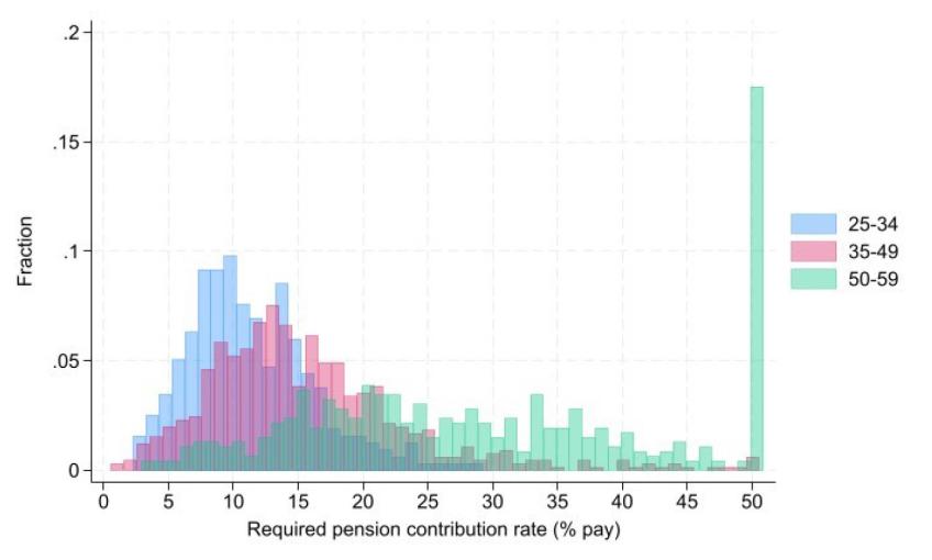
Note: The sample contains 25- to 59-year-old private sector employees saving into a DC pension in Round 7 of the Wealth and Assets Survey. We simulate the share of income they need to save to reach target replacement rates under our baseline assumptions, modelling everyone at the individual level and without accounting for future housing costs or inheritances. The graph shows a histogram of required saving rates for those who are projected to not reach their target replacement rate under their current saving rate.
Figure 4.14. Distribution of required pension contribution rates to achieve PLSA minimum retirement living standard among those currently not on track to achieve target, by age group
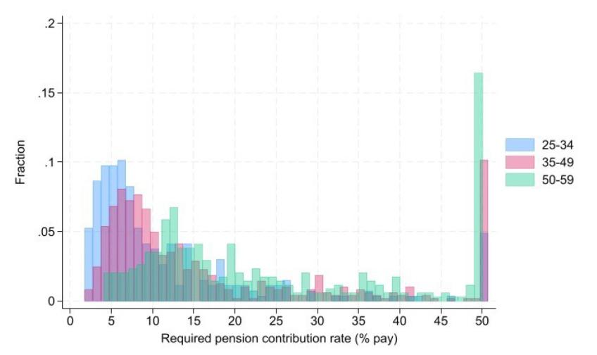
Note: The sample contains 25- to 59-year-old private sector employees saving into a DC pension in Round 7 of the Wealth and Assets Survey. We simulate the share of income they need to save to reach the PLSA minimum retirement living standard under our baseline assumptions, modelling everyone at the individual level and without accounting for future housing costs or inheritances. The graph shows a histogram of required saving rates for those who are projected to not reach the PLSA minimum retirement living standard under their current saving rate.
The second thing to highlight from these two figures is that there is substantially more variation in required saving rates for older workers than for younger workers. In fact, almost 20% of those aged between 50 and 59 who are projected to miss their target replacement rates would need to save over 50% of their income between now and retirement to reach them. As discussed, this is because older workers have many fewer years over which to change their saving in order to reach adequacy and because there is much variation in the pension wealth they have accumulated to date.
Up to now, we have focused on our baseline model results. Table 4.4 shows that these results are sensitive to some of the assumptions we have made on the rates of return, the value of the state pension, and the possibility of using an inheritance to fund your retirement living standards.
Table 4.4. Percentage of private sector employees saving into a DC pension who are projected to hit different measures of retirement income adequacy, by group, in upside and downside scenarios
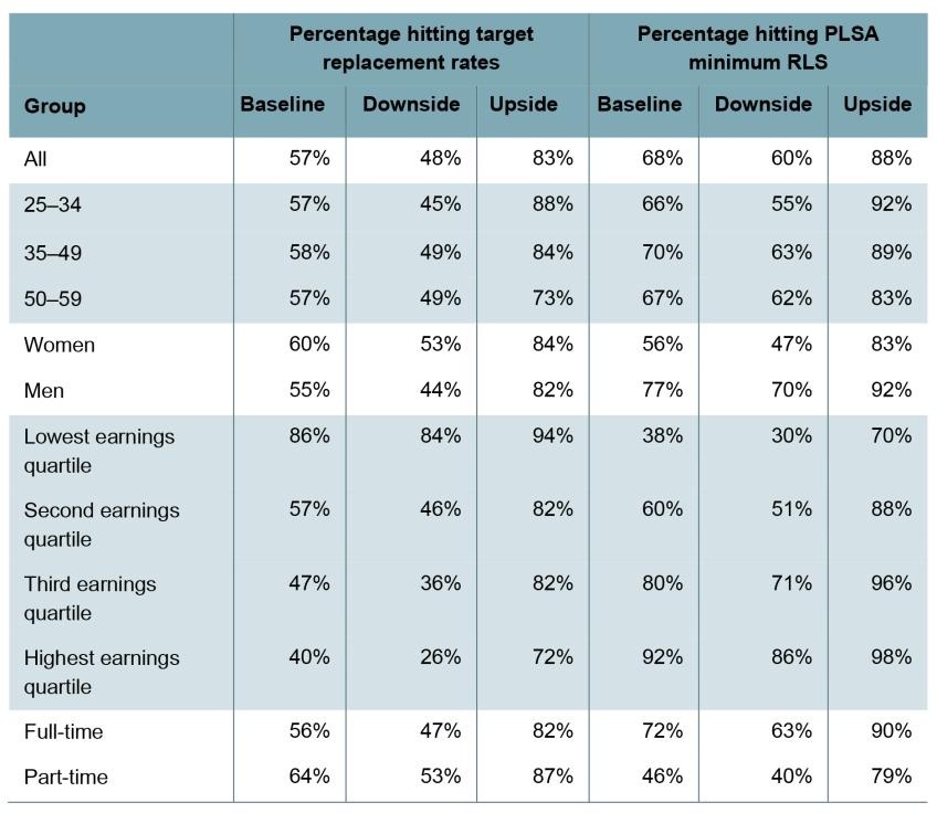
Note: RLS = retirement living standard. The sample contains 25- to 59-year-old private sector employees saving into a DC pension in Round 7 of the Wealth and Assets Survey. We simulate their projected future retirement income under two scenarios and then calculate the share achieving each measure of adequacy. Downside scenario: rates of return (in accumulation and decumulation) are 1 percentage point lower. Upside scenario: rates of return are 1 percentage point higher, and additionally the value of the state pension is 10% higher and we incorporate inheritances. Earnings quartiles are based on pre-retirement earnings, i.e. simulated average earnings between ages 50 and 59.
The ‘Downside’ columns show the shares reaching each measure of adequacy when the rates of return during the accumulation phase and the decumulation phase are both 1 percentage point lower than in the baseline scenario, at 2.3% and 0.3% respectively (in real terms). The ‘Upside’ columns show the shares reaching adequacy when the rates of return are both 1 percentage point higher than in the baseline (at 4.3% and 2.3% respectively), when the value of the state pension is 10% higher, and when we include inheritances in the modelling. More detail on the modelling of inheritances is given in Bourquin, Joyce and Sturrock (2020) and detail on how we include them in our retirement income modelling is given in Section A.8, with the empirical distribution of modelled values of inheritances given in Figure A.1 in Appendix A. Overall, 12% of our sample are not modelled to receive an inheritance, with a further 26% modelled to receive an inheritance worth at most £10,000. Among everyone else, the median inheritance received is worth around £225,000.
Reducing the rate of return in the downside scenario reduces the share reaching each measure of adequacy by slightly under 10 percentage points compared with the baseline. The reduction in adequacy shares is particularly large for younger workers due to the fact that they would face these lower rates of return for longer. When looking at the target replacement rate metric, the reduction in adequacy shares is particularly large among higher earners, for whom private saving represents a higher share of their retirement income.
The proportions meeting each measure of adequacy are substantially higher in the upside scenario with a higher rate of return, a more generous state pension and the inclusion of inheritances. In this scenario, 83% of people are projected to be on track to reach their target replacement rate and 88% on track to reach the PLSA minimum retirement living standard. All groups analysed have shares reaching adequacy for both metrics of over 70%. This emphasises that the modelling results are very sensitive to assumptions about the saving context, especially about the rate of return on saving and the potential for future inheritances to fund retirement living standards in the future.
4.4 Results accounting for partners, the costs of private renting and inheritances
The results in the previous section modelled everyone as an individual; however, in reality of course many people when in retirement will live with others who might have accumulated a rather different amount of retirement wealth. As a result, in this section we focus our attention on those aged 35–59, starting at 35 because of difficulties associated with modelling whether or not they will become part of a couple – and, if so, with whom. We therefore assume that those currently in a (cohabiting or married) couple will remain in a couple into retirement and will share their resources equally between each other. Overall, almost 80% of our sample are living as a couple, with this share slightly higher among men, those below age 50 and higher earners. Among people in a couple, 87% have a partner who is in paid work at the time of the survey and 70% have a partner who is saving into a pension.
In recent years, several reports have raised concerns that a higher share of future retirees might live in private rented accommodation and have low living standards in retirement (Pensions Policy Institute, 2023; Cribb et al., 2023b). We therefore also account for this in this section. To do so, we first simulate the extent to which those currently renting privately will remain in the private rented sector in retirement, and then assume that future private renters will spend the same share of income in retirement on rent as we observe them spending on rent in the Wealth and Assets Survey.
Figure 4.15 shows that around 10% of our sample are projected to live in private rented accommodation in retirement. In comparison, under 7% of people aged over 65 in the 2021 England and Wales census were living in private rented accommodation.15 This share is slightly higher among those in the bottom half of the pre-retirement income distribution and particularly high among single people, at almost 20%. Among those who are projected to live in private rented accommodation in retirement, the mean share of income spent on rent is 24%.
Figure 4.15. Percentage of private sector employees currently saving in a DC scheme who are projected to be single or a private renter in retirement, by group

Note: The sample contains 35- to 59-year-old private sector employees saving into a DC pension in Round 7 of the Wealth and Assets Survey. The green bars show the percentages who are single today, which we assume is also the percentage who will be single in retirement. The yellow bars show the percentage projected to live in private rented accommodation in retirement. Earnings quartiles are based on pre-retirement earnings, i.e. simulated average earnings between ages 50 and 59.
Table 4.5 shows how the share of individuals over age 35 who are projected to be on track to meet their target replacement rates changes when we model people at the couple level. The penultimate column then adds in housing costs for the group of people modelled to rent privately in retirement, while the final column further adds in projected future inheritances and assumes these are entirely used to fund spending in retirement.
Table 4.5. Percentage of private sector employees aged 35–59 saving into a DC pension who are projected to hit target replacement rates, by group and specification
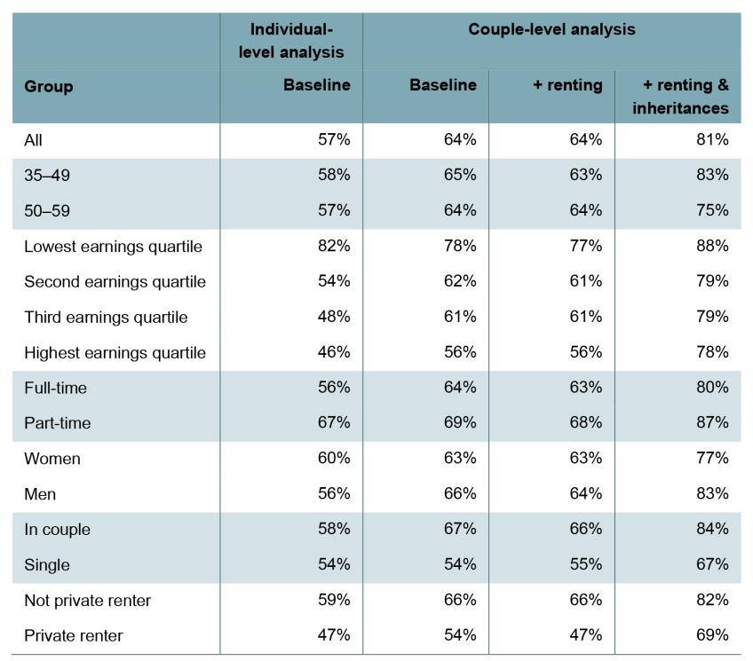
Note: The sample contains 35- to 59-year-old private sector employees saving into a DC pension in Round 7 of the Wealth and Assets Survey. We simulate their projected future retirement income under our baseline economic assumptions. We then compare future retirement incomes with the income needed to achieve their target replacement rate. The first column shows the results when everyone is modelled at the individual level. The next column instead models couples jointly, assuming they share their incomes. The next column also incorporates housing costs for those living in private rented accommodation in retirement. The final column also includes the effects of future inheritances, assuming that these are entirely used to fund spending in retirement. Earnings quartiles are based on pre-retirement earnings, i.e. simulated average earnings between ages 50 and 59.
Overall, modelling people at the couple level rather than the individual level increases the share projected to reach their target replacement rates by 7 percentage points. Of course, the share of single people projected to hit their target replacement rates is by construction unchanged, while we see a 9 percentage point increase in the adequacy share among people who are in a couple. Interestingly, we see a fall in adequacy for individuals in the bottom quartile of pre-retirement earnings, while we see an increase in adequacy for those in the higher quartiles. This occurs because those in the bottom quartile tend to have a higher-earning partner, meaning that their household is better off on average than the original individual. Given that higher earnings are associated with a lower probability of reaching target replacement rates, this reduces the share projected to hit adequacy in the bottom quartile of the pre-retirement earnings distribution. We see the opposite effect higher up the pre-retirement earnings distribution as these people are more likely to have a lower-earning partner.
In the penultimate column of Table 4.5, we project forward whether households will rent privately in retirement. For those households who we forecast to rent privately, we assume that the share of their income they spend on rent in future periods will be the same as the share they currently spend on rent, and we account for any future housing benefit they might receive.
For our whole sample, incorporating the cost of renting into the analysis has almost no impact on the share projected to hit their target replacement rate – it falls by less than 1 percentage point. The main reason for this is that only a minority of our sample – around 10% – are projected to rent in the private sector in retirement. When focusing in on this sample of future private renters, the share projected to achieve their target replacement rate falls from 54% to 47% when we account for the cost of renting. Even this reduction is relatively modest. This is because these individuals are also projected to rent privately during their 50s, and so their pre-retirement income (after housing costs) is low, reducing the target income they have to aim for in retirement. This demonstrates that those who are likely to rent privately when in retirement will also typically have lower living standards while of working age, meaning that substantially increasing their retirement saving may not be affordable for many.
In the final column of Table 4.5, we additionally include inheritances in the analysis as before. Again, this significantly increases the fraction who are projected to reach their target replacement rates, from 64% to 81%. While this is a big increase, it reflects the very large resources that many are likely to receive through a substantial inheritance combined with the (strong) assumption that all of those inherited resources are used for people’s own retirement resources, rather than – for example – being passed on to younger generations. There are two groups who stand out as being less likely to be on track to reach this measure of adequacy even in this specification: single people and future private renters. For both these groups, around one-third are still modelled to miss their target replacement rates.
In Table 4.6, we show the same analysis as in Table 4.5 but focusing on the share projected to reach the PLSA minimum retirement living standard. Single people’s retirement income is compared with the (gross value) of the retirement living standard for single people, while for couples their combined income as a couple is compared with the standard for couples.
Table 4.6. Percentage of private sector employees aged 35–59 saving into a DC pension who are projected to hit the PLSA minimum retirement living standard, by group and specification
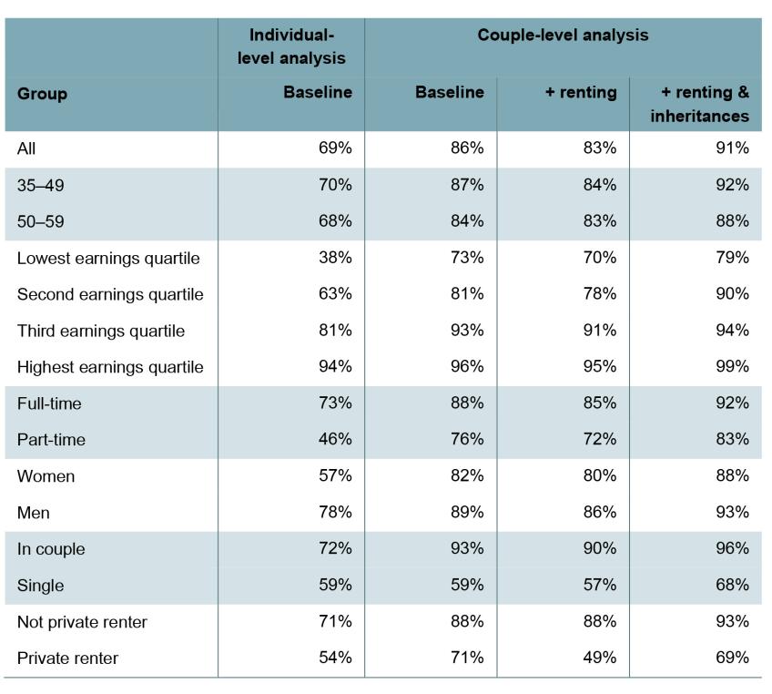
Note: The sample contains 35- to 59-year-old private sector employees saving into a DC pension in Round 7 of the Wealth and Assets Survey. We simulate their projected future retirement income under our baseline economic assumptions. We then compare future retirement incomes with the PLSA minimum retirement living standard (which is uprated with average earnings growth). The first column shows the results when everyone is modelled at the individual level. The next column instead models couples jointly, assuming they share their incomes. The next column also incorporates housing costs for those living in private rented accommodation in retirement. The final column also includes the effects of future inheritances. Earnings quartiles are based on pre-retirement earnings, i.e. simulated average earnings between ages 50 and 59.
Table 4.6 demonstrates that modelling people when incorporating partners’ incomes substantially increases the share projected to hit the PLSA minimum retirement living standard, from 69% to 86% overall. All groups experience an increase in this adequacy share, except, of course, single people, for whom modelling at the couple level changes nothing.
The increases in the share reaching this adequacy metric are particularly large for those groups with lower shares reaching adequacy initially at the individual level. The adequacy share among those in the bottom quartile of the pre-retirement earnings distribution approximately doubles, from 38% to 73%, while the adequacy share for the top quartile increases by only 2 percentage points, from 94% to 96%. The share of women reaching this PLSA standard increases by 25 percentage points, from 57% to 82%, while for men the share increases by 11 percentage points, from 78% to 89%. Broadly, this pattern reflects that lower earners (and women, who are more likely than men to be lower earners) quite often have a higher-earning partner which, if resources are shared, helps them reach the PLSA standard.
Adding on renting costs for future private renters again has little effect on the overall share reaching the PLSA standard – it falls by only 3 percentage points, from 86% to 83%. However, once we focus in on future private renters, we see a much more significant fall in the share reaching this adequacy metric, from 71% to 49%. This is a larger fall than we saw when incorporating renting costs in Table 4.5 because we do not reduce the level of the PLSA living standard to account for the fact that future private renters will also have lower disposable income when in working life due to housing costs.
Incorporating inheritances again pushes up the shares reaching the PLSA minimum retirement living standard. Overall, in this version of the model, over nine in ten people are projected to hit the PLSA minimum retirement living standard. Similar to when comparing with the target replacement rate adequacy measure, the two groups that stand out for having low rates meeting the PLSA standard are single people and future private renters. Again, almost one-third of both these groups are projected to miss the PLSA living standard. Given that we get this consistent picture when comparing with both adequacy measures, despite their differences, both these groups should be of particular concern for policymakers when it comes to their future retirement living standards.
Figures 4.16 and 4.17 show how far away people’s future projected retirement incomes are from the PLSA minimum living standards and their target replacement rate retirement income, respectively. In Figure 4.16, we plot the empirical cumulative distribution function of retirement incomes (combining income together for couples), after housing costs (and housing benefit) but before tax. The dashed vertical lines show the (gross) PLSA minimum retirement living standards for single people and couples. In Figure 4.17, we plot the ratio of the projected retirement income to the retirement income (incorporating the partner’s income) they need to achieve their target replacement rate. In both figures, we include the impact of future housing costs but not inheritances.
Figure 4.16. Distribution of projected retirement incomes (combined incomes for couples) among private sector employees aged 35–59 saving into a DC pension, by marital status

Note: The sample contains 35- to 59-year-old private sector employees saving into a DC pension in Round 7 of the Wealth and Assets Survey. We simulate their projected future retirement income under our baseline assumptions, combining income for couples and accounting for housing costs for future private renters. The graph then plots the empirical cumulative distribution function of retirement incomes, deflated to 2023 by average earnings growth, separately for single people and those in a couple. The dashed vertical lines show the value of the (pre-tax) PLSA minimum retirement living standards. We limit the horizontal axis to values from 0 to £60,000.
Figure 4.17. Distribution of ratio of projected retirement income (combined income for couples) to replacement-rate-target retirement income among private sector employees aged 35–59 saving into a DC pension, by marital status
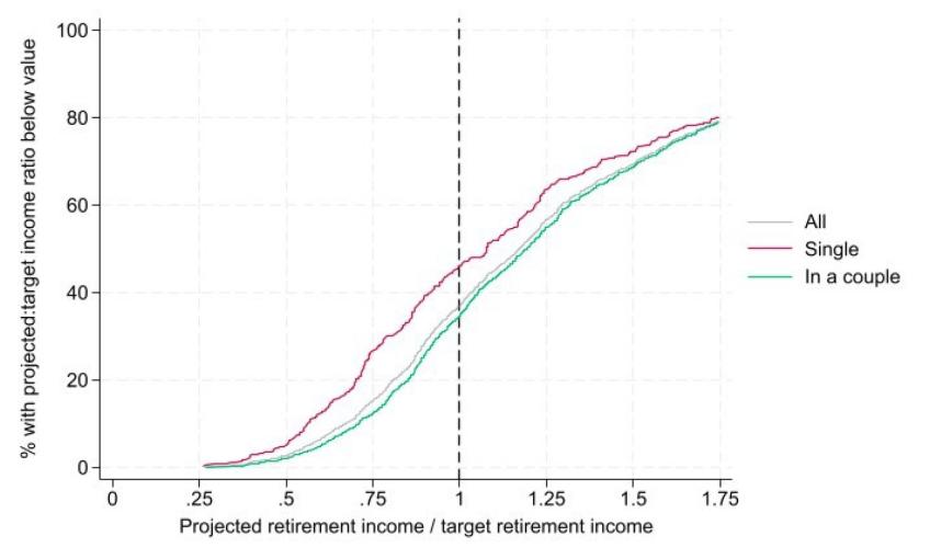
Note: The sample contains 35- to 59-year-old private sector employees saving into a DC pension in Round 7 of the Wealth and Assets Survey. We simulate their projected future retirement income under our baseline assumptions, combining income for couples and accounting for housing costs for future private renters. The graph then plots the empirical cumulative distribution function of projected retirement income divided by target retirement income (based on replacement rates and again combined for couples), separately for single people and those in a couple. We limit the horizontal axis to values from 0.25 to 1.75.
In this version of the model, not only do most people in couples reach the PLSA minimum living standard, but a sizeable proportion are actually quite far above it. For example, almost 25% of people in couples have a pre-tax household retirement income of over £60,000. Over 40% of people in couples reach the PLSA moderate retirement living standard. Around two-thirds of people in couples are projected to achieve their target replacement rate, although slightly over 10% will have a retirement income at least 25% lower than that needed to reach their target replacement rate.
Single people tend to be further away from hitting their measures of adequacy. Around 10% of this group have to leave work before state pension age and do not have enough pension wealth accumulated to have incomes as high as the value of the state pension before they reach state pension age. A quarter of single people are projected to have a retirement income at least 25% lower than that needed to reach their target replacement rate. Nevertheless, a substantial minority of single people still seem to be on track to achieve a replacement rate much higher than their target: around a fifth of single people are projected to have a retirement income over 75% above their replacement rate target income.
We also extend the modelling by incorporating other types of saving and wealth into the analysis. Modelling saving into several different asset classes throughout the entirety of employees’ working lives is beyond the scope of this report. Instead, we take 50- to 59-year-olds, who have already accumulated a significant share of their non-pension wealth, and show the effects of incorporating their non-pension and non-primary-residence wealth into the analysis on the shares projected to reach adequacy. The results are shown in Figure B.1 in Appendix B. Accounting for these other sources of wealth leads to relatively modest increases in the shares projected to meet adequacy measures of under 10 percentage points. This stands in stark contrast to results for the self-employed, where accounting for other types of wealth increases adequacy measures by up to 20 percentage points (Cribb et al., 2024b). This highlights that private pension wealth is a much more important source of retirement income for employees than for the self-employed.
4.5 Summary
Overall, our modelling suggests that while the majority of private sector employees currently saving into a DC pension are on track to have an adequate income in retirement, there is a substantial minority who seem to be ‘undersaving’. In our baseline model for all ages, we project that 43% of private sector employees in a DC pension are not on track to achieve their target replacement rate (around 7 million people) and 32% are not on track to hit the PLSA minimum retirement living standard (around 5 million people). However, these results are sensitive to some of the assumptions underlying the modelling, in particular regarding the rate of return on saving, the use of future inheritances to fund retirement, and whether we model people as individuals or at the household level.
Certain groups appear more likely to be undersaving than others. Higher earners are more likely to be undersaving than lower earners when comparing with the target replacement rate measure of adequacy, with the reverse being true when comparing with the PLSA minimum retirement living standard. Modelling people at the household level, rather than as individuals, moderates these patterns with regards to earnings somewhat, as higher earners often have a lower-earning partner and lower earners often have a higher-earning partner and therefore assuming that resources are shared within couples tends to even out the patterns by earnings. The share of employees who are projected to be undersaving does not vary significantly with age; however, older employees who are undersaving often need to save much higher proportions of their earnings to reach adequacy than younger employees who are undersaving. This is both because there is significant variation in the situation of older employees – some of whom have spent many years saving in defined benefit pensions, while others have not saved much in a pension at all – and because older employees have fewer years left to make up for low levels of past saving.
Two groups that stand out as being particularly likely to be undersaving, regardless of the assumptions used in the modelling, are single people and those living in private rented accommodation in retirement. Even modelling at the household level and assuming people will use future inheritances to fund their retirements, around one-third of both these groups are projected to be undersaving relative to both adequacy measures. However, both of these groups tend to have both lower incomes and higher spending pressures during working life, potentially making large increases in pension saving unaffordable for many. One final group to mention is the set of employees who are not currently saving into a pension. They are not included in our main analysis sample due to greater uncertainty about how their pension contribution rate may change in the future; however, there are clearly concerns that many in this group might be undersaving for retirement too.
5. What level and timing of saving are recommended by an economic model?
The analysis of the previous chapter gave us an insight into where retirement incomes are heading on current trends and what saving rate would be required to hit adequacy. This analysis tells us how much different groups would need to save, under certain assumptions, in order to hit their benchmark replacement rates or the PLSA minimum retirement living standard. However, it does not tell us whether it is a good idea for savers to be aiming to hit those measures of adequacy, nor when in their lives would be the best time to save.
In this chapter, we use an economic model of saving to shed light on how much and when people should save. The model builds on that presented in Crawford, O’Brien and Sturrock (2021) and the interested reader can consult that report for a more detailed description of the model. In essence, the model is an economic ‘life-cycle’ model where an individual aims to smooth their material living standards over their lifetime by saving into, and subsequently drawing on, a private pension. As in the modelling undertaken in Chapter 4, all individuals are assumed to receive a full new state pension from state pension age onwards.
A key advantage of this model, compared with other analytical tools, is that it takes seriously the trade-offs that individuals face when making saving decisions – most notably, that additional saving out of take-home pay now will lead to higher income and consumption in retirement (which is valuable) at the cost of lower consumption today (which is costly). As in most economic models of saving and consumption, it assumes that additional consumption is more valuable when you have low levels of consumption (i.e. the ability to spend an extra £100 per year is more valuable if you currently spend £10,000 per year than if you currently spend £50,000 per year). This means that, when making the trade-off between consumption today and consumption in retirement (by saving for the future), the trade-off will be different depending on whether you are likely to be richer or poorer in retirement than you are today.
Individuals in this model face uncertainty over their future earnings and longevity and they respond to the economic incentives given by returns to saving and the tax and student loan repayment systems when choosing when to save and spend. They face costs that vary over their life course due to the arrival of children. We update the model to be consistent with the modelling assumptions in this report (most importantly around earnings growth, the level of the state pension, rates of investment return on assets, and life expectancy). This model is stylised. For example, it considers people as making individual saving decisions with no reference to the resources or needs they may have through having a partner. In addition, to help us understand whether each stage of life is a good point to be transferring resources to retirement, we abstract from the fact that for most employees, participating in a private pension scheme requires minimum contributions that, assuming they are made, allow individuals to receive at least a small employer contribution.16 The model therefore needs to be looked at within context and alongside other evidence. However, it can give us some useful insights into how saving should vary between groups and over the life course.
Figure 5.1 shows the median simulated saving rate recommended by the model for different groups over working life. In the model, low earners typically do not make contributions to a private pension until they reach their 50s. This reflects the fact that they will choose to save only when their standard of living is at least as high as they expect it to be in retirement. Generally speaking, those with higher earnings will tend to save more, consistent with the analysis in Chapters 3 and 4, but this model gives stark conclusions about when this saving should take place.
Figure 5.1. Simulated median optimal saving rate from the life-cycle model for each third of the contemporaneous earnings distribution, split by sex
Panel A. Men
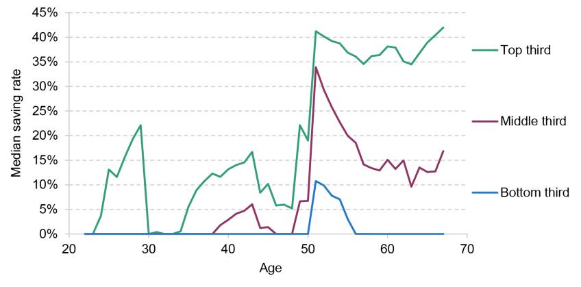
Panel B. Women
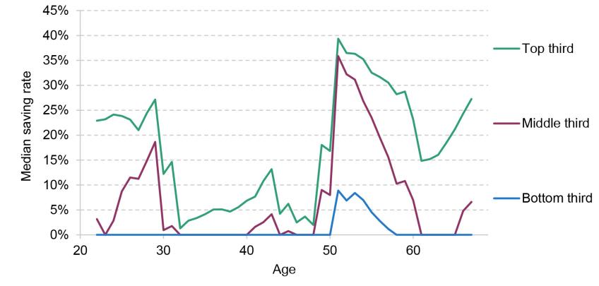
Note: The graphs show the median saving rate at each age for people in the top, middle and bottom thirds of the contemporaneous earnings distribution, separately for men and women. They are based on outputs from an economic life-cycle model, where we simulate earnings and optimal saving rates over the life cycle for 1,000 example individuals.
Those in the middle and top thirds of the earnings distribution are simulated to increase their saving dramatically after age 50, when their costs are assumed to fall (due to children leaving home and their student loan being paid off) and their earnings are highest. The rates of saving predicted by the model at these ages are very high – up to 40% for the highest-earning men. Saving is also relatively high when people are in their 20s, before children have arrived (we assume two children are born, the first at age 30 and the second at age 32). It is important to note that this model does not account for saving for a house deposit, which would make it less favourable to save in a pension at these ages. Women earning in the middle and top thirds save more than their male counterparts in early adult life. This is because their earnings do not tend to grow as steeply as men’s through later working life.
Overall, these results highlight that saving rates ought to vary as circumstances change over the life cycle, with there being several reasons to save more in later working life. As shown in Crawford, O’Brien and Sturrock (2021), this finding remains even if assuming high rates of return to pension saving (7%), and hence a greater value to saving early to benefit from the compounding of returns.
However, underlying these average optimal saving rates there is considerable variation in what people are simulated to choose to save, even when comparing people at the same age and with the same level of earnings. In the model, this can happen because they will have had a different history of saving due to different levels of earnings in the past and because they may have different levels of expected earnings growth in the future. In the real world, there are myriad reasons why those who have the same level of earnings might appropriately make different saving choices. Pensions policy must be set bearing in mind the potential for a wide variety of personal situations and will inevitably be balancing the risks of undersaving and oversaving.
With this point in mind, Figure 5.2 shows selected points of the distribution of saving rates from the model, split by decile of current earnings, where deciles are defined across the whole working-age population. It is only in the top half of the earnings distribution that the median person (P50) is saving. That said, in the sixth decile (just above average), a quarter of people are predicted to optimally save at least 15% of their earnings, and this climbs to a quarter of people having saving rates of at least 20% in the eighth decile. While saving is very concentrated among individuals with higher levels of earnings, because people will move around the earnings distribution over the course of their lives, a much larger share of people will be optimally accumulating some retirement savings over their whole working life than are saving at one point in time. Alternatively put, although this model suggests that those outside of the top half of current earnings should rarely save for retirement, this does not mean that those in the bottom half of the lifetime earnings distribution should not accumulate retirement savings. It means that people with moderate lifetime earnings should only be doing their retirement saving at the times in their lives when they have relatively high earnings (and low costs).
Figure 5.2. 25th, 50th and 75th percentiles of life-cycle saving rates, by decile of current earnings
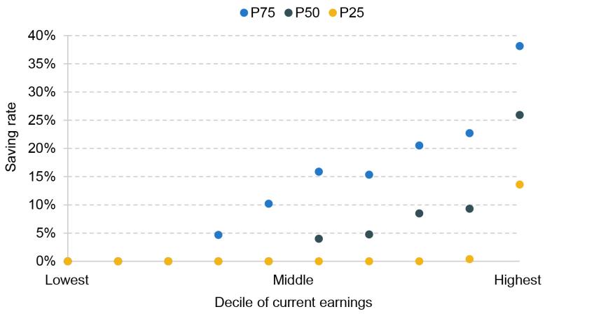
Note: This graph shows the 25th, 50th and 75th percentiles of saving rates separately for each decile of the current earnings distribution. It is based on outputs from an economic life-cycle model, where we simulate earnings and optimal saving rates over the life cycle for 1,000 example individuals.
While the stylised nature of this model means its quantitative findings are a loose guide rather than an exact prescription, it would suggest that any increases in automatic enrolment default total contribution rates should be focused on those in the top half, and perhaps even the top quartile, of the earnings distribution, if they are to serve the purpose of smoothing living standards over the whole of life. In addition, the fact that earnings are relatively high and costs relatively low in later working life suggests that a policy that increased default rates at some later age, such as 50, could have some merit.
6. Conclusion
Much has changed since the Pensions Commission reported around 20 years ago. On the one hand, there have been substantial boosts in the level and the coverage of the flat-rate part of the state pension, giving people a firmer foundation upon which to build their private savings. On the other hand, depressed returns to saving coupled with lower prospects for earnings growth have made the saving landscape more challenging. Taking these changes together, we calculate that someone spending their lifetime as a low, middle or high earner would have to have a higher saving rate to hit the targets set out by the Pensions Commission, by around 1–3% of earnings.
Of course, in reality, people do not spend all their life at the same point in the earnings distribution – they instead move up and down the distribution, and potentially spend several years out of paid work. And there is significant dispersion in the amount of pension wealth that today’s employees have already accumulated, even for people of similar ages with similar levels of earnings today.
In this report, we therefore undertake new modelling of the retirement income prospects of today’s employees, taking into account their saving to date and how their earnings and employment status could be expected to evolve in the future. We do this for a representative sample of private sector employees currently saving in defined contribution pensions, to shed light on whether today’s savers as a whole seem to be on track for an adequate level of income in retirement. Importantly, we also go beyond the overall picture and show the distribution of future simulated retirement incomes, highlighting which groups seem particularly likely to be on track for inadequate income in retirement. Based on these modelling results, in the accompanying report (Cribb et al., 2024a) we assess different potential reforms to automatic enrolment and make concrete recommendations on how to improve the system for employees. We also repeat the modelling analysis for self-employed workers and discuss potential policy recommendations for this group in Cribb et al. (2024b).
Overall, in our baseline model, we project that over half (57%) of current private sector employees saving in a defined contribution pension are on track to meet their target replacement rate in retirement, while around two-thirds (68%) are on track to meet the PLSA minimum retirement living standard. Importantly, though, these estimates are by nature sensitive to some of the assumptions in the model – in particular, around the rate of return on saving, whether we include the impact of future inheritances, and the decision on whether to model people at the individual level or to combine income for couples.
However, despite this uncertainty, we find that certain groups consistently appear more likely to be undersaving than others under a variety of different modelling assumptions. For example, higher earners appear less likely to be on track to hit their replacement rate than lower earners, as the state pension on its own replaces a significant share of lower earners’ pre-retirement earnings. In contrast, lower earners appear more likely than higher earners to have retirement income below the level of the PLSA minimum retirement living standard. However, many working families today currently also have incomes below the level of this income standard, implying that it might not be appropriate to encourage more private saving among this group. Rather, to the extent that policymakers wish to boost the retirement incomes of lifetime low earners, this would be best done via further redistribution towards them to avoid eroding their current low living standards. Helping more lifetime low earners to remain in paid work up to (or beyond) the state pension age would also improve their retirement living standards.
Two other groups that stand out as having low levels of retirement income adequacy are single people and private renters in retirement. People who are single in retirement cannot benefit from sharing resources and costs and are projected to be significantly less likely than people in couples to achieve the PLSA minimum living standard (57% compared with 90%) and their target replacement rates (55% compared with 66%). Those projected to live in private rented accommodation in retirement have lower rates of adequacy than those who are not privately renting as they have higher costs in retirement. This difference in adequacy rates is more pronounced when comparing with the PLSA minimum living standard than when comparing with the target replacement rates measure, given that the latter measure accounts for the fact that private renters in retirement tend to be private renters during working life as well, and so have lower disposable income out of which to do their saving.
The final group to highlight is the group of employees who are not currently saving into a pension. We do not include them in our main modelling results; however, there are clearly concerns about whether they should be saving more for retirement. Despite the success of automatic enrolment in increasing pension participation, we still find that over a quarter of private sector employees are not saving into a pension, half of whom are targeted by automatic enrolment and half not.
The policy suggestions we make in our accompanying report (Cribb et al., 2024a) build on these modelling results together with other pieces of evidence. We discuss how automatic enrolment can work better for the significant group of employees who are not saving in a pension currently, the key trade-offs around increasing retirement incomes for lower earners, and how to ensure that higher earners are transferring enough of their income to retirement given they are particularly unlikely to be on track to achieve their target replacement rates.
Appendix A. Modelling future retirement incomes
A.1 Summary of modelling approach
In this appendix, we provide more details on our modelling of future retirement incomes of the current working-age population, based on data from Round 7 of the Wealth and Assets Survey.
At a high level, the model first involves estimating future pension saving for each individual, based on simulations of their future employment status and earnings. We then calculate retirement incomes, based on this future projected saving together with any saving they have already done by the time of the survey, and other sources of income – most importantly, the state pension. These retirement incomes are then compared with the PLSA minimum retirement living standard and with an income target based on the target replacement rates set out by the Pensions Commission.
In this appendix, we provide more detail on these calculations, in particular how we:
- simulate future earnings;
- estimate the periods when individuals are out of paid work;
- estimate the age at which an individual permanently leaves the labour market;
- model future pension saving;
- calculate retirement incomes;
- calculate the target retirement incomes.
We extend the baseline model in a variety of ways to show the sensitivity of our results. We describe the following in this appendix:
- how we model the future receipt of inheritances and how this affects retirement incomes assuming all inheritances are used to finance retirement;
- how we model retirement incomes and adequacy at the couple (‘benefit-unit’) level;
- how we model who will be a private renter in retirement;
- how we model adequacy for future private renters;
- how we incorporate other, non-pension, sources of wealth in the modelling.
Finally, we discuss the assumptions we make in our baseline model about economic growth, rates of return and other economic parameters.
A.2 Simulating future earnings
For each individual in our analysis sample (a subset of 25- to 59-year-olds in paid work), we observe in the Wealth and Assets Survey their earnings, age, sex and education level. These are the starting points for our earnings simulation. We then want to simulate how much the individual will earn in each future year until they reach retirement. We also simulate ‘backwards’ earnings in previous years, as these can be important both for calculating retirement incomes (in particular from defined benefit pensions) and for defining the retirement income target based on target replacement rates.17
We simulate earnings based on processes estimated using the British Household Panel Survey and its successor, Understanding Society. Our estimation method has two broad steps. First, we estimate age profiles of average log earnings for each sex, education and 10-year birth cohort group. This tells us how earnings for those in work tend to change with age for each group. The specification is the same as used in Sturrock (2023). For further details, see that paper. We adjust the growth rate of earnings such that it is consistent with a 1.8% annual growth rate in future years. The second step accounts for how earnings vary around that average. From the data, we have a distribution of deviations of earnings from the group-specific average. We employ the method of Arellano, Blundell and Bonhomme (2017) to estimate the distribution of transitions between points in this distribution, as a function of the individual’s position in the earnings distribution within their group. The process for these transitions is estimated separately by sex-and-education group.
We thus obtain two key ingredients needed for our earnings simulation. First, we obtain estimates of the distribution of earnings for each year, age, sex, education level and generation. Second, we obtain estimates of the probability of moving from one point of the earnings distribution to another point from one year to the next for each age, sex, education level and starting point in the earnings distribution.18 These processes are first-order Markov processes in the sense that we assume the probability of being at a certain point in the earnings distribution in the next year only depends on where the individual is in the earnings distribution in the current year, i.e. it does not depend on where they were in the earnings distribution in previous years. We also back out the estimated probability of having moved from one point of the earnings distribution in the previous year conditional on where they are in the distribution in the current year.
Then, armed with these tools, we take where each individual is in the earnings distribution in the starting period from the Wealth and Assets Survey, simulate forwards, and backwards, their position in the earnings distribution in all years back to when they were age 25 and up to the year before reaching state pension age. And we can use the estimates of the earnings distribution in all these years to obtain, for each individual, their level of annual earnings in each year of working life should they be in paid work in this period. Table B.2 in Appendix B compares levels of earnings in the starting period with average earnings between ages 50 and 59, and shows there is a non-negligible amount of earnings mobility in our modelled earnings profiles.
A.3 Simulating periods out of work up to age 59
Working-age people spend time out of paid work for a variety of reasons, which will affect their accumulation of pension wealth. To account for this, we simulate movements into and out of paid work using processes estimated using Waves 1–12 of Understanding Society. Our sample for this estimation is respondents aged between 25 and 59. We estimate these processes as follows.
We first estimate the probability of moving from paid work in one year to not being in paid work the following year. To do this, we take the sample of observations where the individual is in paid work in a given wave but not retired in the following wave. We then run a probit model regression to estimate the probability of the respondent not being in paid work in the following wave and how this varies by generation, education, age group and sex.19
We also estimate the probability of moving from being out of paid work in one year to being in paid work in the following year. For this, we use the sample of observations where the individual is not in paid work in a given year and drop anyone who is retired in the given year, in any of the past two years or in the next year. We then run a probit model regression to estimate the probability of the respondent not being in paid work in the following wave and how this varies by generation, education, age group, sex and also the length of time they have been out of paid work for (either one year, two years or at least three years). We also derive the probabilities to simulate movements backwards in time.
In the starting period (i.e. when we observe people in the Wealth and Assets Survey), everyone in our sample is in paid work. We then use the estimated probabilities of moving into and out of paid work to simulate whether the individual is in paid work or not for all future years up to age 59 and for all previous years back to age 25. For any period in which we model someone as out of paid work, they receive no earnings and do no pension saving.
A.4 Estimating when people permanently leave work
At some point in our model, people leave work permanently never to return, and start to draw on their accumulated wealth to fund their retirement.
Our starting assumption is that people retire at state pension age. In reality, people might permanently stop working at an earlier age for several reasons. Some people have little choice over the matter – for example, if they have health problems that force them to retire, or if they lose their job and find themselves unable to find a new one, or if they have to give up work to care for a relative. In contrast, some people might choose to retire early because they think they can afford to do so and still enjoy a comfortable retirement. This behaviour is important to account for, as Cribb (2023) shows that people retiring before state pension age are disproportionately wealthy, but people who are out of work for other reasons prior to state pension age have disproportionately low levels of wealth.
When modelling when people leave work, we want to model exits before state pension age due to health problems, caring responsibilities and job losses. These are often unexpected and can mean people have to draw on their accumulated pension wealth earlier than they might have been planning to. On the other hand, we do not conceptually want to capture exits due to the choice to take early retirement. This is to avoid the case where someone would have reached a given measure of adequacy if they had worked until state pension age, but they choose to retire earlier than this and consequently have a lower retirement income which falls short of the adequacy measure. Given this was a choice to retire early and have lower retirement income, we do not want to measure this as ‘inadequate’. For a similar intuition, we also do not allow people to work past state pension age. Working past state pension age would increase someone’s retirement income, making them more likely to meet a given adequacy benchmark; however, there is a cost to retiring later (principally lower leisure time) and we do not want to be labelling people’s retirement saving as adequate just because they retire in their mid 70s.
We therefore model labour market exits before state pension age in two ways. First, if someone is out of work at age 59 (based on the simulations described in Section A.3), we assume that they do not return to work in their 60s. For everyone else in the simulation, we model whether they leave work between age 60 and the year before they reach state pension age based on probabilities estimated from the Labour Force Survey. To estimate these, we take people born in either 1956 or 1957 in this dataset and calculate for six education-by-sex groups the increase in the share of people out of work due to unemployment or long-term sickness between the ages of 50 and 64. We then divide these numbers by 14 (as we measure changes over a 14-year period) to get an estimate of the share of people leaving work in each year due to unemployment or long-term sickness in each group. Then, for each age from 60 to the year before state pension age, we take this share as the probability that an individual from each group leaves work permanently at this age. Overall, around 13% of our full sample (people in the Wealth and Assets Survey aged between 25 and 59 and in paid work) are modelled to leave paid work before state pension age. Table A.1 shows that the probability of leaving paid work before state pension age is higher for women than for men, and for those with lower levels of formal education.
Table A.1. Shares modelled to leave paid work before state pension age, by sex and education level
| Education level | Sex | Share leaving paid work before state pension age |
| Up to GCSEs | Men | 15% |
| Up to GCSEs | Women | 19% |
| A levels | Men | 12% |
| A levels | Women | 14% |
| Degree or equivalent | Men | 6% |
| Degree or equivalent | Women | 12% |
Note: This table shows the percentage of our sample (including both self-employed and private sector employees saving in DC pensions) who are modelled to permanently leave paid work before state pension age.
A.5 Modelling future pension saving
For all years where the individual is in paid work, we assume that they continue to save into their pension at the same rate as in the initial year (when we observe them in the Wealth and Assets Survey).
To be precise, for those who are saving into a defined contribution pension in the survey, we assume that they continue to save into a defined contribution pension with the same contribution rate as in the survey (measured as a proportion of total earnings). For those who are saving into a defined benefit pension in the survey, we assume that they stay in this scheme for all years when they are in paid work and that there is no change in scheme rules. Finally, for anyone who is not saving into a private pension in the survey, we assume that continues to be the case in any future years.
In reality, many people will change their pension contribution rate over time, and some will move into and out of pension saving over time. As a result, our estimates should not be thought of as giving a perfectly realistic prediction of each individual’s future private pension wealth. Instead, we are extrapolating current saving behaviour to project future retirement incomes based on current saving trends.
A.6 Calculating retirement incomes
First, we need to determine when to calculate retirement incomes. There are several options here. For example, we could take average income over all periods after an individual permanently leaves work, or we could take the average over all periods after an individual reaches state pension age, or we could measure income over a more limited set of periods.
We choose to define an individual’s retirement income as their income in the first year after they have permanently left work (by construction, this will be between ages 60 and 68). There are two advantages to this choice. First, it is simpler to calculate. Second, and more importantly, it is a conservative choice, as real income is weakly increasing during retirement in our model, as we explain below. In other words, with this choice, our results give a lower bound on people’s retirement incomes.
The next question is how to calculate an individual’s income in the first year after permanently leaving work (call this age a ̂ ). We start with any benefits the individual is entitled to – either the state pension (which is uprated in line with average earnings growth) if a ̂ is equal to their state pension age, or working-age benefits if a ̂ is before state pension age (which we set to be the value of jobseeker’s allowance and uprate in line with inflation). On top of this, we assume that the individual starts to receive their defined benefit (DB) pension at age a ̂, and add this on to their income.20
The final ingredient is the total amount of non-DB private wealth the individual has accumulated at age a ̂, call this W, coming from all their defined contribution pension saving as well as any extra wealth from inheritances or other sources of non-pension wealth (as explained in Sections A.8 and A.12). If a ̂ is state pension age, we assume that the individual purchases a (CPI) inflation-linked annuity with all of W (how we calculate annuity income is described below). If a ̂ is before state pension age, we assume they draw down W in such a way that their total income in each year before state pension age is equal to their income once they reach state pension age (when they again purchase an annuity with any remaining wealth). If W is not large enough to achieve this, we instead assume they draw down all of W before state pension age so that they have equal income in all these years. To calculate annuity income from a pot of wealth, we assume that annuities are actuarially fair based on cohort-by-gender life expectancy estimates (Office for National Statistics, 2024) and a rate of return (1.8% in real terms in the baseline model).
As a result, real incomes weakly increase after age a ̂. This is for two reasons. First, if a ̂ is before state pension age, then if an individual does not have high enough non-DB private wealth to smooth their income between age a ̂ and state pension age, their income will increase upon reaching state pension age. Second, we assume that the state pension is indexed to average earnings growth (assumed to be 1.8% per year in real terms). As a result, people’s state pension income increases each year after state pension age in real terms. Since we assume they buy an inflation-linked annuity with W, their total income therefore also increases during retirement in real terms.
A.7 Calculating target retirement incomes
We use two measures of a target, ‘adequate’, retirement income throughout our analysis. The first is the PLSA minimum retirement living standard, set at £14,400 annually for single people in 2023/24.21 Given this is an expenditure target, we transform this into a pre-tax income target (assuming that parameters of the tax system are indexed to average earnings growth) given that the rest of our modelling is for pre-tax incomes. We assume that this target increases in line with average earnings growth (1.8% per year in real terms) over time, implying that what is considered to be a minimum standard of living in retirement rises as overall national living standards rise.
The second target is calculated by taking a measure of pre-retirement income and multiplying it by a ‘target replacement rate’. The target replacement rates were first produced by the Pensions Commission in 2004; we uprate their income bands by average earnings growth since then, giving us the target replacement rates shown in Table A.2. We calculate pre-retirement income as average income between ages 50 and 59, made up of earnings as well as universal credit for low earners. For simplicity, we always model universal credit receipt at the individual level (ignoring children), and we assume that the maximum value of the universal credit is uprated in line with earnings, while the taper rate on post-tax earnings remains 55%.
Table A.2. Target replacement rates (TRRs) and pre-retirement income bands
| Pre-retirement income band | Pensions Commission (2004) | BHC thresholds, 2023 earnings | BHC TRR | AHC thresholds, 2023 earnings | AHC TRR |
| Band 1 (lowest) | Less than £9,500 | Less than £17,000 | 80% | Less than £14,500 | 84% |
| Band 2 | £9,500–17,499 | £17,000–31,499 | 70% | £14,500–27,999 | 75% |
| Band 3 | £17,500-24,999 | £31,500–44,999 | 67% | £28,000–40,999 | 71% |
| Band 4 | £25,000–49,999 | £45,000–89,999 | 60% | £41,000–82,499 | 63% |
| Band 5 (highest) | £50,000 and more | £90,000 and more | 50% | £82,500 and more | 53% |
Note: Pre-retirement income is defined to be average income between ages 50 and 59 inclusive (including universal credit for low earners). We uprate the BHC (before-housing-cost) income thresholds used by the Pensions Commission (2004) by growth in average earnings to obtain the BHC thresholds in 2023. To obtain the AHC (after-housing-cost) thresholds, we uprate the thresholds used in Department for Work and Pensions (2023) by factors consistent with the difference between our BHC thresholds and DWP’s.
A.8 Modelling inheritance receipt
Previous research at IFS (Bourquin, Joyce and Sturrock, 2020) has shown that inheritances are set to make up a larger proportion of lifetime incomes for younger generations than for their predecessors. Given that they are, on average, received at around age 60, they could be an important source of income for future generations of retirees. As a result, we provide a model extension where we model the receipt of future inheritances and assume that all these inheritances are used to fund retirement spending (as opposed to funding long-term care needs or bequests). Throughout, we focus on modelling inheritances received from parents, as these are by far the largest source of inheritances for most people (Boileau and Sturrock, 2023).
The Wealth and Assets Survey contains some data on whether the respondent has already received an inheritance from their parents. For those respondents who are in all waves of the survey, we can observe whether they have ever received a parental inheritance. If they have, then we do not allow them to receive another one, to avoid double counting. For respondents who we do not observe in all previous waves of the survey, we have information on whether they received a parental inheritance back to a certain age, a ̃, but not before this. We then simulate whether they had received a parental inheritance before age a ̃ using the probability of having done so modelled by Bourquin, Joyce and Sturrock (2020). These probabilities vary by generation and education level.
For everyone who has not yet (or is simulated to have not yet) received a parental inheritance by the time of survey, we model the amount of inheritance they will receive in the future. To do this, we again make use of estimates from Bourquin, Joyce and Sturrock (2020). They provide estimates of the distribution of parental inheritances by generation and education level. Note that this distribution includes zeros for those who will not receive a parental inheritance. To use these estimates, we first, for simplicity, assume that all inheritances are received at age 60.22 Then, to assign inheritances to future recipients, we first take the set of respondents whose parents are not homeowners, and give them an inheritance from the bottom quintile of the distribution of inheritance receipt. For everyone else, we randomly assign them an inheritance from the top 80% of the distribution of inheritance receipt for their education level and generation. The distribution of the modelled value of received inheritances is shown in Figure A.1.
Figure A.1. Distribution of modelled values of received inheritances
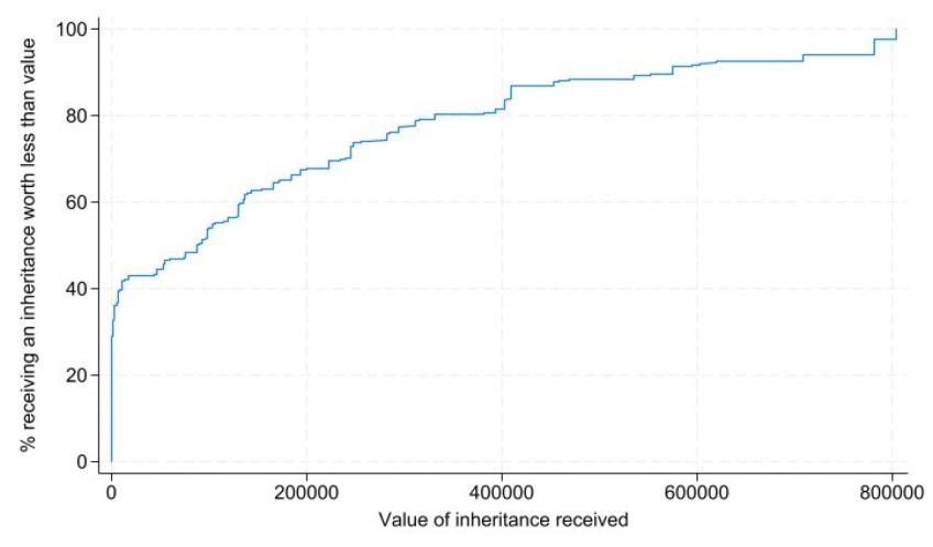
Note: This figure displays the empirical cumulative distribution function of modelled inheritances received for full sample of 25- to 59-year-old workers in the Wealth and Assets Survey. The graph shows, for each inheritance value (shown on the horizontal axis), the percentage of our sample who receive an inheritance worth less than this value (shown on the vertical axis).
We then assume people use all their received inheritance to fund their retirement, as set out in Section A.6. Note that because we model the probability of inheriting at the individual level, single people can receive at most one inheritance over their lifetime, and couples can receive at most two inheritances (one from each set of parents).
A.9 Modelling at the couple level
We also show how our results change if we model retirement incomes at the couple level (for those people who are married or cohabiting), rather than the individual level.
To model retirement incomes at the couple level, we first have to determine who will be in a couple at the point they reach retirement. Given the difficulties associated with modelling the formation and dissolution of relationships, for simplicity we restrict our sample to those aged at least 35 and assume that the couples we observe in the survey will last until retirement. We choose the age of 35 because the share of people living with a spouse/partner is relatively stable from this age onwards, as shown in Figure A.2. Therefore, although we will evidently misclassify some people as having a partner in retirement who actually split up before then, and will misclassify others as being single in retirement even though they find a partner in the meantime, on average our estimates should give a good idea of people’s relationship status by the time they reach retirement. Around 80% of individuals aged at least 35 in our analysis sample are in a couple in the survey (and therefore also at retirement).
Figure A.2. Share of individuals who are married or cohabiting by age, 2019
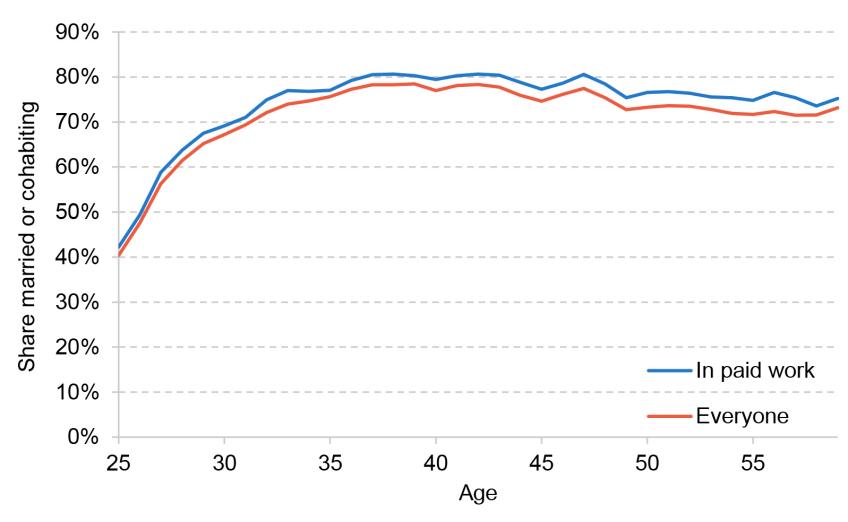
Source: Authors’ calculations using the Labour Force Survey.
For single people, our calculations of their retirement income and how this compares with their target is then as in Section A.6. The calculations change for people with a spouse/partner as follows. We set the age at which we calculate a couple’s retirement incomes as the first year after which both members of the couple are assumed to have permanently left paid work. We then calculate both total retirement income for the couple in this year and equivalised retirement income (which is the amount a single person would require to reach the same standard of living, i.e. total retirement income for the couple divided by 1.67).
We then compare total retirement income for the couple with measures of retirement income adequacy for the couple. For the PLSA minimum retirement living standard, we use the (pre-tax) version of the standard, uprated by earnings to the year in which we measure retirement incomes (i.e. for couples, the first year after both members of the couple have left work). For the ‘target replacement rate’ income measure, we add together average individual income between ages 50 and 59 for both members of the couple to get pre-retirement income. We multiply this by the relevant target replacement rate, based on equivalised retirement income (as in Table A.2), to get the retirement income target.
A.10 Modelling who will be a private renter in retirement
Private renters in retirement face considerably higher housing costs than both homeowners and social renters. Those born in the 1970s and, especially, the 1980s have been considerably more likely to live in private rented accommodation than earlier generations at the same age (Cribb et al., 2023b), prompting concerns that they will also be more likely to rent privately in retirement, face higher housing costs, and potentially need higher incomes to enjoy an ‘adequate’ standard of living (Pensions Policy Institute, 2023).
There is of course uncertainty about how many people among future generations of retirees will be in private rented accommodation, and who these people will be. This is particularly true for the youngest generations; as a result, we restrict our attention to those aged at least 35 when accounting for how private renting affects our results.
We then need to model who will be a private renter in retirement among those aged at least 35 in our sample. We assume first that anyone in the survey who is at least age 45 and lives in private rented accommodation will also do so once they reach retirement. This is because, for previous generations, the share renting privately levels out from around age 45 (Cribb et al., 2023b).
For those aged between 35 and 44, we assume that some people who are in private rented accommodation at the time of the survey will move into homeownership (or social housing) by the time they reach retirement. In particular, we assume that the share of private renters in this generation falls from 19.5% at the time of the survey to match the share who are private renters among those born in the early 1970s at the time of the survey, 13%.
Our simulations of who in this age group moves out of private rented accommodation are based on probabilities estimated from Understanding Society. We create a longitudinal panel of waves 1–12 of the survey and estimate the probability of someone in private rented accommodation in one wave remaining in private rented accommodation the next year by their marital status, their quartile of (equivalised) benefit-unit earnings and their region using a probit model. We then scale these probabilities such that we obtain the share of private renters we are aiming for among 35- to 44-year-olds.
A.11 Modelling retirement income adequacy among private renters
To account for the fact that private renters in retirement might need a different amount of income to have an adequate standard of living, we modify the two measures of retirement income adequacy as follows.
The PLSA retirement living standards are designed to reflect the expenditure that retirees might need assuming they are both mortgage- and rent-free. As a result, for people we project to live in private rented accommodation in retirement, we assume that they spend the same share of their income on rent during retirement as the share we observe them spending in the WAS survey period and add this resulting rent during retirement on to the PLSA retirement income target. We then also reduce the income target by the amount of housing benefit the individual might expect to receive. We approximate the maximum amount of housing benefit that someone might expect to receive today by calculating the 30th percentile of annual rents among one-bedroom dwellings for each government office region in the Wealth and Assets Survey. We assume this is uprated in line with average earnings growth to get the maximum potential housing benefit entitlement for each region at the point we are measuring retirement incomes, and then subtract the amount of housing benefit from the target to get the BHC, pre-housing-benefit, minimum retirement living standard, appropriately taking into account tapering.
To modify the ‘target replacement rate’ income measure, we follow the Department for Work and Pensions (2023). We calculate pre-retirement income after housing costs (AHC) and housing benefit during people’s 50s, use the target replacement rates for AHC income shown in Table A.2 to calculate target AHC retirement income, and then add on rents and subtract housing benefit to obtain the BHC (before-housing-costs) and pre-housing-benefit income target.
A.12 Incorporating non-pension wealth
Pensions are not the only way in which people can save for retirement. We therefore provide an extension to the model where we incorporate non-pension wealth. However, we cannot observe the share of income someone is saving in non-pension assets in the Wealth and Assets Survey, making it difficult to model non-pension saving flows.
Therefore, for this model extension, we restrict our attention to people aged between 50 and 59, who in general have already accumulated a large proportion of their non-pension wealth, and ignore any further accumulation of these types of wealth past these ages. This will underestimate the amount of non-pension wealth people have upon reaching retirement if people do accumulate much more wealth between the survey and retirement; on the other hand, we assume that people use all their non-pension wealth for funding living standards in retirement, which will offset this underestimate.
We take the value of different forms of non-pension wealth each individual has at the time of survey, uprate it to the year in which we measure their retirement income, and then add this on to their total non-DB wealth and calculate retirement incomes as in Section A.6.23 Note that we do not include main-property wealth in this analysis. The annual rates of return used to uprate non-pension wealth are shown in Table A.4 later, where we also assume fees of 50 basis points a year for all assets except cash and money market investments, and a long-term annual inflation rate of 2%. In addition, we assume a rate of return on business wealth of 1.8% per year in real terms, consistent with the growth rate of average earnings.
A.13 Baseline economic assumptions
Since we are modelling future retirement incomes, we have to make assumptions about how a set of economic variables will evolve over the future. Our main assumptions are shown in Table A.3. We assume that average economy-wide earnings growth will be 1.8% per year in real terms in the future, consistent with OBR forecasts (Office for Budget Responsibility, 2024). We assume that the state pension will be indexed in line with this growth in average earnings, consistent with the recommendations made in Cribb et al. (2023a) for the future of the state pension.
Table A.3. Assumptions on main economic parameters
| Parameter | Assumption |
| Average annual real economy-wide earnings growth | 1.8% |
| Real rate of return per year on saving during the accumulation period | 3.3% |
| Real rate of return per year obtained by annuity providers | 1.8% |
| Indexation of the state pension | Average earnings growth |
Note: Average annual real economy-wide earnings growth rate assumption is from Office for Budget Responsibility (2024). Assumptions on real rates of return are based on assumed rates of return for underlying assets in Table A.4. We assume earnings indexation of the state pension, in line with the recommendations made in Cribb et al. (2023a).
To obtain an assumption on the rate of return on pension saving during the accumulation period, we follow the methodology in the original Pensions Commission (2004) report and calculate this based on assumptions about the typical asset allocation mix of pension schemes together with assumptions on expected returns for these underlying assets. These assumptions can be found in Table A.4.
Table A.4. Assumptions on rates of return for different asset classes, and the assumed share of pension saving portfolio they constitute during the accumulation period
| Asset | Assumed nominal rate of return | Portfolio share |
| Government bonds | 4.5% | 20% |
| Corporate bonds | 5.3% | 10% |
| Equities | 6.5% | 60% |
| Property | 5.5% | 7% |
| Cash and money market investments | 1.5% | 3% |
| Overall nominal rate of return, before fees | 5.8% | |
| Overall nominal rate of return, after fees (of 50 basis points) | 5.3% | |
| Overall real rate of return | 3.3% |
Note: The portfolio shares come from Financial Conduct Authority (2017), as do the assumed nominal rates of return on equities, property, and cash and money market investments. The nominal rates of return for bonds are based on nominal forward gilt curves. The fees are consistent with findings from Department for Work and Pensions (2020).
The portfolio shares in Table A.4 come from Financial Conduct Authority (2017), as do the expected rates of return on equities, property, and cash and money market investments. We assume a nominal rate of return on government bonds of 4.5% in the long term, consistent with UK instantaneous nominal forward gilt curves,24 and keep a spread of corporate bonds over UK gilts of 0.8%, consistent with Financial Conduct Authority (2017). We also assume average fees of 50 basis points based on Department for Work and Pensions (2020), and a long-run inflation rate of 2% consistent with the Bank of England target. Putting this together gives an overall real rate of return assumption of 3.3% during the accumulation period. For comparison, the Department for Work and Pensions (2023) assumes an average nominal rate of return before fees are subtracted of 5.75%, very similar to our assumption of 5.8%. DWP assumes that fees are drawn from a distribution with a maximum value of 75 basis points.
To obtain the expected rate of return for annuity providers, we follow the Pensions Commission (2004) and subtract 0.7 percentage points from the expected rate of return on government bonds (to account for fees and profits) to obtain a nominal rate of return of 3.8%. The real rate of return for annuity providers is therefore 1.8%.
Appendix B. Additional figure and tables
Table B.1. Replication of table 4.10 of first Pensions Commission report
| Age | Earnings (2004 terms) | Pensions Commission numbers | Our replication |
30 40 50 60 | £9,000 £9,000 £9,000 £9,000 | 0% 0% 1% 4% | 1% 3% 3% 4% |
30 40 50 60 | £21,250 £21,250 £21,250 £21,250 | 8% 8% 7% 6% | 11% 10% 9% 8% |
30 40 50 60 | £50,000 £50,000 £50,000 £50,000 | 8% 7% 6% 5% | 9% 8% 8% 7% |
Note: Authors’ calculations updating Pensions Commission (2004) analysis for an individual starting to save at age 25 and working until state pension age. Earnings are assumed to grow at a constant rate each year. The individual is assumed to save a constant fraction of their earnings in each year in order to reach their target replacement rate (80% for the lower earner, 67% for the middle earner and 50% for the higher earner). Our modelling comes very close to replicating the Pensions Commission’s numbers.
Figure B.1. Effect of including other types of accumulated wealth in modelled adequacy for private-sector employees aged between 50 and 59 who are saving in a DC pension
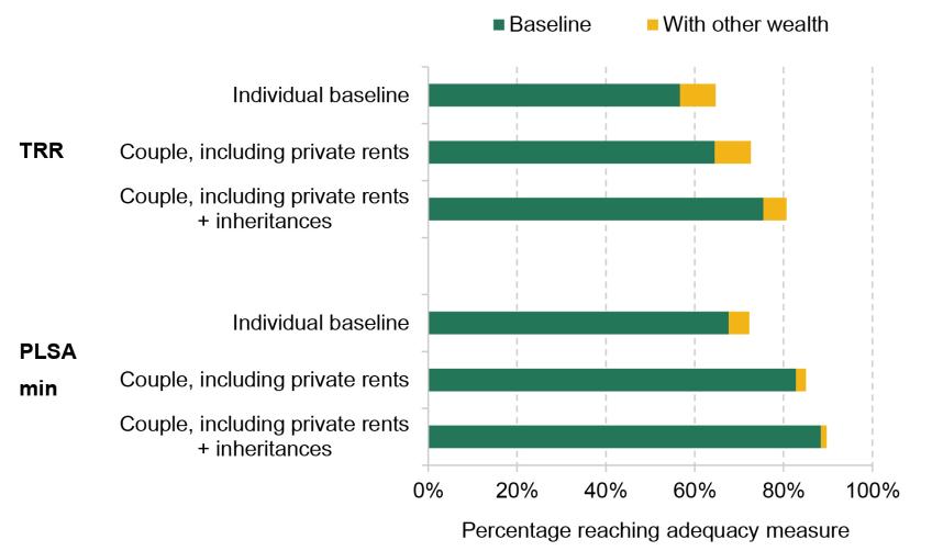
Note: The graph shows the share of 50- to 59-year-old private sector employees saving in a DC pension who are projected to achieve their target replacement rate (TRR) or the PLSA minimum retirement living standard (PLSA min). The green bars show the percentage meeting these measures of adequacy when only including (state plus private) pension income, while the yellow bars show the extra percentage meeting adequacy when also allowing people to accumulate retirement wealth in non-main properties, financial assets and businesses. We show this for our individual baseline model, and also show the effects of including partners’ income and future housing costs, and also including inheritances.
Table B.2. Percentage of employees in different quartiles of age 50–59 earnings, by current earnings quartile and age group
| Age group | Quartile of current earnings | Quartile of age 50–59 earnings | |||
| Q1 | Q2 | Q3 | Q4 | ||
25–34 25–34 25–34 25–34 | Q1 Q2 Q3 Q4 | 35% 28% 18% 21% | 33% 23% 20% 23% | 18% 27% 29% 27% | 15% 22% 34% 29% |
35–49 35–49 35–49 35–49 | Q1 Q2 Q3 Q4 | 46% 29% 14% 11% | 27% 32% 23% 18% | 19% 24% 29% 27% | 8% 14% 33% 44% |
50–59 50–59 50–59 50–59 | Q1 Q2 Q3 Q4 | 75% 21% 3% 1% | 21% 57% 20% 2% | 3% 19% 57% 21% | 2% 3% 20% 76% |
Source: Authors’ calculations using Round 7 of the Wealth and Assets Survey.
Table B.3. Percentage of employees who are projected to hit different measures of retirement income adequacy, by group, for those currently saving in a defined benefit pension, and for private sector employees not currently saving in a defined benefit pension
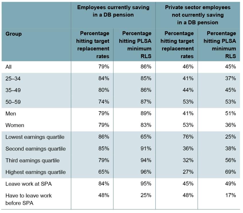
Note: RLS = retirement living standard. SPA = state pension age. ‘Employees currently saving in a DB pension’ includes public sector employees. ‘Private sector employees not currently saving in a DB pension’ includes both participants in DC schemes and those not participating at all. Both are samples of 25- to 59-year-olds.
Source: Authors’ calculations using Round 7 of the Wealth and Assets Survey.
Appendix C. Advisory group membership
Age UK
Citizens Advice
Confederation of British Industry (CBI)
Department for Work and Pensions (DWP)
Federation of Small Businesses (FSB)
Financial Conduct Authority (FCA)
Generation Rent
HM Revenue & Customs (HMRC)
HM Treasury (HMT)
Institute and Faculty of Actuaries (IFoA)
Institute for Government (IfG)
Joseph Rowntree Foundation (JRF)
Lane Clark & Peacock LLP (LCP)
Money and Pensions Service (MaPS)
NEST Insight
Pensions and Lifetime Savings Association (PLSA)
Pensions Policy Institute (PPI)
Resolution Foundation
The Association of British Insurers (ABI)
The Behavioural Insights Team (BIT)
The International Longevity Centre (ILC-UK)
The Pensions Regulator
The Runnymede Trust
Trades Union Congress (TUC)
Which?
References
Adrjan, P. and Bell, B., 2018. Pension shocks and wages. Centre for Economic Performance, Discussion Paper 1536, https://cep.lse.ac.uk/pubs/download/dp1536.pdf.
Aguiar, M. and Hurst, E., 2005. Consumption versus expenditure. Journal of Political Economy, 113, 919–48, https://doi.org/10.1086/491590.
Arellano, M., Blundell, R. and Bonhomme, S., 2017. Earnings and consumption dynamics: a nonlinear panel data framework. Econometrica, 85, 693–734, https://doi.org/10.3982/ECTA13795.
Association of British Insurers, 2022. Automatic enrolment: what will the next decade bring? https://www.abi.org.uk/globalassets/files/publications/public/lts/2022/automatic-enrolment-what-will-the-next-decade-bring/.
Banks, J., Blundell, R. and Tanner, S., 1998. Is there a retirement-savings puzzle? American Economic Review, 88, 769–88, http://www.jstor.org/stable/117005.
Binswanger, J. and Schunk, D., 2012. What is an adequate standard of living during retirement? Journal of Pension Economics and Finance, 11, 203–22, https://doi.org/10.1017/S1474747211000618.
Boileau, B. and Sturrock, D., 2023. Who gives and receives substantial financial transfers in Britain? Institute for Fiscal Studies, Working Paper 23/08, https://ifs.org.uk/publications/who-gives-and-receives-substantial-financial-transfers-britain.
Bourquin, P., Joyce, R. and Sturrock, D., 2020. Inheritances and inequality within generations. Institute for Fiscal Studies, Report 173, https://ifs.org.uk/publications/inheritances-and-inequality-within-generations.
Broome, M., 2024. Calculating a Living Pension: the 2024 update. Resolution Foundation, https://www.resolutionfoundation.org/app/uploads/2024/09/Living-pension.pdf.
Cominetti, N. and Odamtten, F., 2022. Living pensions: an assessment of whether workers’ pension saving meets a ‘living pension’ benchmark. Resolution Foundation, https://www.resolutionfoundation.org/app/uploads/2022/07/Living-Pensions.pdf.
Crawford, R., O’Brien, L. and Sturrock, R., 2021. When should individuals save for retirement? Predictions from an economic model of household saving behaviour. Institute for Fiscal Studies, Report BN326, https://ifs.org.uk/publications/when-should-individuals-save-retirement-predictions-economic-model-household-saving.
Crawford, R. and O’Dea, C., 2012. The adequacy of wealth of those approaching retirement. Institute for Fiscal Studies, Report 72, https://ifs.org.uk/publications/adequacy-wealth-among-those-approaching-retirement.
Cribb, J., 2023. Understanding retirement in the UK. Institute for Fiscal Studies, Report 284, https://ifs.org.uk/publications/understanding-retirement-uk.
Cribb, J. and Emmerson, C., 2020. What happens to workplace pension saving when employers are obliged to enrol employees automatically? International Tax and Public Finance, 27, 664–93, https://doi.org/10.1007/s10797-019-09565-6.
Cribb, J., Emmerson, C., Johnson, P. and Karjalainen, H., 2023a. The future of the state pension. Pensions Review, Institute for Fiscal Studies, https://ifs.org.uk/publications/future-state-pension.
Cribb, J., Emmerson, C., Johnson, P., Karjalainen, H. and O’Brien, L., 2023b. Challenges for the UK pension system: the case for a pensions review. Institute for Fiscal Studies, Report 255, https://ifs.org.uk/publications/challenges-uk-pension-system-case-pensions-review.
Cribb, J., Emmerson, C., Johnson, P., O’Brien, L. and Sturrock, D., 2024a. Policies to improve employees’ retirement resources. Institute for Fiscal Studies, Report 332, https://ifs.org.uk/publications/policies-improve-employees-retirement-resources.
Cribb, J., Emmerson, C., O’Brien, L. and Sturrock, D., 2024b. Private pensions for the self-employed: challenges and options for reform. Institute for Fiscal Studies, Report 330, https://ifs.org.uk/publications/private-pensions-self-employed-challenges-and-options-reform.
Cribb, J., Karjalainen, H. and O’Brien, L., 2023. The gender gap in pension saving. Institute for Fiscal Studies, Report 250, https://ifs.org.uk/publications/gender-gap-pension-saving.
Department for Work and Pensions, 2013. The single-tier pension: a simple foundation for saving. https://assets.publishing.service.gov.uk/media/5a7b622940f0b64646935cb1/single-tier-pension.pdf.
Department for Work and Pensions, 2017. Automatic Enrolment Review 2017: maintaining the momentum. https://www.gov.uk/government/publications/automatic-enrolment-review-2017-maintaining-the-momentum.
Department for Work and Pensions, 2020. Pension charges survey 2020 – summary. https://www.gov.uk/government/publications/pension-charges-survey-2020-charges-in-defined-contribution-pension-schemes/pension-charges-survey-2020-summary.
Department for Work and Pensions, 2023. Analysis of future pension incomes.https://www.gov.uk/government/statistics/analysis-of-future-pension-incomes/analysis-of-future-pension-incomes.
Financial Conduct Authority, 2017. Rates of return for FCA prescribed projections. https://www.fca.org.uk/publication/research/rates-return-fca-prescribed-projections.pdf.
Finch, D. and Pacitti, C., 2021. Building a Living Pension. Resolution Foundation, https://www.resolutionfoundation.org/app/uploads/2021/01/Building-a-living-pension.pdf.
HM Revenue and Customs, 2024. Private pension statistics: table 6. https://www.gov.uk/government/statistics/personal-and-stakeholder-pensions-statistics.
Hurman, N., Jethwa, C., Pike, T. and Silcock, D., 2021. What is an adequate retirement income? Pensions Policy Institute, https://www.pensionspolicyinstitute.org.uk/media/lbwo3ojh/20210609-adequate-retirement-income-final.pdf.
Jordà, Ò., Knoll, K., Kuvshinov, D., Schularick, M. and Taylor, A. M., 2019. The rate of return on everything, 1870–2015. Quarterly Journal of Economics, 134, 1225–98, https://doi.org/10.1093/qje/qjz012.
Mayhew, V., 2002. Pensions 2002: public attitudes to pensions and saving for retirement. DWP Research Report 193.
Office for Budget Responsibility, 2023. Fiscal risks and sustainability – July 2023. https://obr.uk/frs/fiscal-risks-and-sustainability-july-2023/.
Office for Budget Responsibility, 2024. Supplementary forecast information release: long-term economic determinants – March 2024. https://obr.uk/supplementary-forecast-information-release-long-term-economic-determinants-march-2024/.
Office for National Statistics, 2022. Employee workplace pensions in the UK: 2021 provisional and 2020 final results. https://www.ons.gov.uk/employmentandlabourmarket/peopleinwork/workplacepensions/bulletins/annualsurveyofhoursandearningspensiontables/2021provisionaland2020finalresults.
Office for National Statistics, 2024. National life tables – life expectancy in the UK: 2020 to 2022. https://www.ons.gov.uk/peoplepopulationandcommunity/birthsdeathsandmarriages/lifeexpectancies/bulletins/nationallifetablesunitedkingdom/2020to2022.
Padley, M., 2024. Retirement living standards in the UK in 2023. Loughborough University, Centre for Research in Social Policy, https://www.retirementlivingstandards.org.uk/2023_research_report.pdf.
Padley, M. and Stone, J., 2023. A Minimum Income Standard for the United Kingdom in 2023. Joseph Rowntree Foundation, https://www.jrf.org.uk/a-minimum-income-standard-for-the-united-kingdom-in-2023.
Pension Protection Fund, 2024. PPF 7800 Index: 30 June 2024. https://www.ppf.co.uk/-/media/PPF-Website/7800/2024/PPF_7800_Update_July_2024.pdf.
Pensions and Lifetime Savings Association, 2022. Five steps to better pensions: time for a new consensus. https://www.plsa.co.uk/Policy-and-Research/Document-library/Five-steps-to-better-pensions-time-for-a-new-consensus.
Pensions and Lifetime Savings Association, 2024. Retirement Living Standards. https://www.retirementlivingstandards.org.uk/.
Pensions Commission, 2004. Pensions: Challenges and Choices: The First Report of the Pensions Commission. The Stationery Office, https://webarchive.nationalarchives.gov.uk/ukgwa/20070801230000/http:/www.pensionscommission.org.uk/publications/2004/annrep/index.html.
Pensions Commission, 2005. A New Pension Settlement for the Twenty-First Century: The Second Report of the Pensions Commission. https://webarchive.nationalarchives.gov.uk/ukgwa/+/http:/www.dwp.gov.uk/publications/dwp/2005/pensionscommreport/main-report.pdf.
Pensions Policy Institute, 2023. The UK Pensions Framework: renting in retirement – the fault line below the UK pension system. https://www.pensionspolicyinstitute.org.uk/research-library/research-reports/2023/2023-11-30-the-uk-pensions-framework-renting-in-retirement-the-fault-line-below-the-uk-pension-system.
Pike, T., 2022. Projection of future pensioner household income, analysis based upon the Wealth and Assets Survey dataset. https://www.pensionspolicyinstitute.org.uk/media/sihnuwdi/20220831-projection-of-pensioner-income-from-was-final.pdf.
Standard Life, 2023. Auto-enrolment: how and when should default contribution rates rise to 12%? https://www.standardlife.co.uk/about/thinking-forward/articles/article-page/auto-enrolment-how-and-when-should-default-contribution-rates-rise-to-twelve-percent.
Sturrock, D., 2023. Wealth and welfare across generations. Institute for Fiscal Studies, Working Paper 23/15, https://ifs.org.uk/publications/wealth-and-welfare-across-generations.
WPI Economics, 2024. Falling behind the curve: the costs of delaying an increase in auto-enrolment contributions – a WPI Economics report for Phoenix Group. https://www.thephoenixgroup.com/media/repp0hoo/falling-behind-the-curve-the-costs-of-delaying-an-increase-in-auto-enrolment-contributions.pdf.
Data
Department for Work and Pensions, NatCen Social Research. (2021). Family Resources Survey. [data series]. 4th Release. UK Data Service. SN: 200017, DOI: http://doi.org/10.5255/UKDA-Series-200017.
Office for National Statistics, Social Survey Division. (2023). Wealth and Assets Survey, Waves 1-5 and Rounds 5-7, 2006-2020. [data collection]. 18th Edition. UK Data Service. SN: 7215, DOI: http://doi.org/10.5255/UKDA-SN-7215-18.
Office for National Statistics. (2024). Annual Survey of Hours and Earnings, 1997-2023: Secure Access. [data collection]. 25th Edition. UK Data Service. SN: 6689, DOI: http://doi.org/10.5255/UKDA-SN-6689-24.
Office for National Statistics. (2024). Labour Force Survey. [data series]. 11th Release. UK Data Service. SN: 2000026, DOI: http://doi.org/10.5255/UKDA-Series-2000026.
University of Essex, Institute for Social and Economic Research. (2023). British Household Panel Survey. [data series]. 3rd Release. UK Data Service. SN: 200005, DOI: http://doi.org/10.5255/UKDA-Series-200005.
University of Essex, Institute for Social and Economic Research. (2024). Understanding Society. [data series]. 12th Release. UK Data Service. SN: 2000053, DOI: http://doi.org/10.5255/UKDA-Series-2000053.
Preface
The abrdn Financial Fairness Trust has supported this project (grant reference 202206-GR000068) as part of its mission to contribute towards strategic change which improves financial well-being in the UK. Its focus is on tackling financial problems and improving living standards for people on low-to-middle incomes. It is an independent charitable foundation registered in Scotland. Co-funding from the ESRC-funded Centre for the Microeconomic Analysis of Public Policy at IFS (grant number ES/T014334/1) is also gratefully acknowledged.
We are grateful for comments and advice from our Steering Group members David Gauke (Chair), Jeannie Drake, David Norgrove and Joanne Segars, from Mubin Haq and Karen Barker at the abrdn Financial Fairness Trust, from Janette Weir from Ignition House and from our Advisory Groups (see list of member organisations in Appendix C). We also benefited from the thoughts of many colleagues, most importantly Carl Emmerson and Paul Johnson, and from conversations with Richard Mosley and Tim Pike.
This work was produced using statistical data from the Family Resources Survey (FRS), the Annual Survey of Hours and Earnings (ASHE), the Wealth and Assets Survey (WAS), Understanding Society (the UK Household Longitudinal Survey, UKHLS), the British Household Panel Survey (BHPS) and the Labour Force Survey (LFS). The FRS data were accessed through an agreement with the Department for Work and Pensions. The ASHE was accessed via the Office for National Statistics’ (ONS)’s Secure Research Service. Data from the WAS and the LFS are Crown Copyright and are reproduced with the permission of the Controller of HMSO and the King’s Printer for Scotland. The WAS is produced by the ONS. The UKHLS and the BHPS are distributed by the UK Data Service. The use of the ONS statistical data in this work does not imply the endorsement of the ONS in relation to the interpretation or analysis of the statistical data. This work uses research data sets which may not exactly reproduce National Statistics aggregates.
Endnotes
Authors

Jonathan Cribb
Jonathan joined IFS in 2011. His research areas includes: pensions, ageing and demographic change, public sector pay, housing, and inequalities.

Laurence O'Brien
Laurence is in the Retirement, Savings and Ageing sector. His work focuses on people’s savings decisions and on economic activity in later life.

More from IFS
Understand this issue


Policy analysis


Academic research


